The expansion of the Universe is now well described by the flat CDM model (). The proportions of each of these components are today evaluated at Planck Collaboration et al. (2020):
In this chapter, we will study the thermal history of the Universe as well as the evolution of its composition. Until now in this course, non-relativistic matter was treated as a single entity, slowing down the expansion of the Universe through its gravitational interaction. But to study its evolution with temperature and its interactions with other components, it is necessary to separate these into two contributions: dark matter and baryonic matter[1] . Indeed, in 1933, while studying the Coma cluster, astrophysicist Fred Zwicky showed that the mass deduced from the motion of the seven galaxies composing it is 400 times greater than the mass deduced from counting luminous objects. This measurement was repeated in 1936 on the Virgo cluster and this time gave a factor of 200. These somewhat imprecise measurements fell into oblivion until the 1970s, when astronomer Vera Rubin observed that the rotation speed of stars in the Andromeda Galaxy is much higher than suggested by its observed luminous mass Rubin & Ford, W. Kent, 1970. The observation was quickly repeated on numerous galaxies: part of the matter constituting the galaxy is therefore dark matter, escaping all detection at the time, often representing the majority of the total mass of galaxies. The presence of abundant dark matter is even visible in the amplitude of temperature anisotropies in the cosmic microwave background (see end of chapter). Today, we estimate that the proportion of these two forms of cold matter is Planck Collaboration et al., 2020:
.
1Description of the primordial Universe
The Cosmic Microwave Background
If the Universe is expanding today, then it was smaller in the past. Cosmic expansion reduces the momentum of particles by a factor and the density of particles by another . In the early times, the Universe was therefore in a hot and dense state. There must therefore have been a moment when the Universe was hot enough for atoms to be ionized, and therefore in a plasma state where photons interact with free electrons. Through these frequent interactions, if thermodynamic equilibrium is reached, the radiation follows a blackbody spectrum defined by the temperature of the medium (wiki:Planck’s_law). During the transition from the plasma state to the neutral state, around for a hydrogen gas, the Universe suddenly becomes transparent and photons propagate freely. This high-temperature blackbody radiation was released at this instant. This so-called fossil radiation has been cooled by the expansion of the Universe. This cosmic microwave background was predicted in 1948 by Ralph Alpher, Robert Herman Alpher & Herman, 1948 and George Gamow Gamow, 1948 around , and discovered fortuitously by Arno Penzias and Robert Wilson in 1964 Penzias & Wilson, 1965Penzias & Wilson, 1965 at a temperature of (Figure 1).
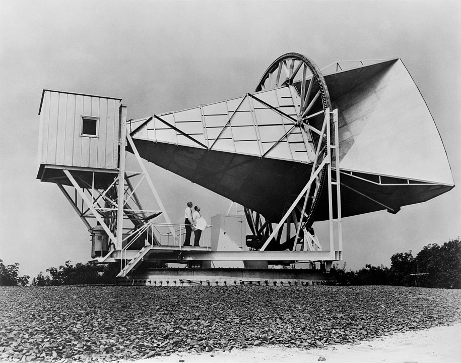
Figure 1:The 15-metre Holmdel horn antenna at Bell Telephone Laboratories in Holmdel, with Arno Penzias and Robert Wilson, which led to the discovery of the CMB. It was built in 1959 as part of work on communications satellites for NASA ECHO I (By NASA, restored by Bammesk).
The spectrum of the cosmic microwave background has been characterized thanks to the COBE satellite, and its temperature is now established at (Fixsen (2009)):
by modeling its data using Planck’s radiation law:
This is the best blackbody radiation ever detected (Figure 2). As we will justify later, if photons interact little with matter, then we can demonstrate that the energy distribution of photons in the past is still a blackbody spectrum, at temperature Condon & Matthews, 2018. So if we go back in time to the last interaction of photons with matter, then at that moment the Universe was in a hotter state than today and at thermal equilibrium, since the radiation followed Planck’s law. The cosmic microwave background radiation (CMB) is probably the most direct evidence that the Universe was indeed in the form of a hot, dense plasma at equilibrium in the distant past.

Figure 2:Fitting a blackbody model to various data measuring the flux from the cosmic microwave background Mather et al., 1999.
Demonstration of the conservation of Planck’s law with redshift

Figure 3:Notations for calculating the evolution of Planck’s law with redshift.
The energy radiance (Radiance) is expressed in W/m/sr. With the definitions of luminosity distance and angular distance, we show that it evolves as . Indeed, with the notations of Figure 3, for a source of luminosity of size , observed under a solid angle , in the small angle approximation:
with the radiance if there were no expansion of space. The observed spectral radiance is expressed in W/m/sr/Hz. All photons received in a small interval around a frequency were emitted in an interval around a frequency . The received radiance is therefore:
We deduce the evolution of the spectral radiance:
Therefore blackbody radiation evolves with redshift as follows:
A blackbody spectrum remains a blackbody spectrum despite the expansion of the Universe but at an equilibrium temperature:
The Universe at redshift 
Let us go back well beyond the redshift of the last scattering surface, and consider the Universe at, say, . What can we say about it?
Temperature
For a photon gas, we know that:
Now, at thermal equilibrium, the energy density of a photon gas is the integral of Planck’s law:
with W/m/K the Stefan-Boltzmann constant. The equilibrium temperature of photons therefore evolves as follows:
The photon temperature can therefore be used as a temporal parameter like or if is isotropic.
At redshift 104, the photon temperature is therefore of the order of K. Hydrogen atoms (which are the majority in the Universe) are therefore necessarily in an ionized state, so the Universe is a plasma.
Evolution of with redshift
Thanks to the few interactions between CMB photons and matter at different redshifts, cosmologists are able to measure the evolution of the temperature of this ambient photon bath with expansion. For example, we can look at the Compton interaction of CMB photons with hot electron plasma () located in galaxy clusters (thermal Sunyaev-Zeldovich effect wiki:Sunyaev–Zeldovich_effect). We can also measure the heating of CO or CN molecules in the interstellar gas by CMB photons at different redshifts. One of the best measurements of the decrease in photon temperature with expansion is with (Hurier et al. (2014), see also Noterdaeme et al. (2011)).
Figure 4:Evolution of CMB photon temperature as a function of redshift, taken from Hurier et al. (2014). The green point corresponds to the COBE measurement. The red points come from tSZ emission from galaxy clusters in the Planck satellite catalog. The blue points come from the study of absorption by the interstellar medium.
Solution to Exercise 1
Densities
We can now calculate the current contribution of CMB photons to the critical density of the universe using the blackbody temperature:
This is therefore a negligible energy density compared to cold matter and dark energy. Certainly, other ultra-relativistic particles such as neutrinos contribute to the remaining part of . But with 3 massless neutrinos, we would only reach as we will see at the end of the chapter.
We define matter-radiation equality as the moment when relativistic and non-relativistic matter are in equal proportion. Let us calculate the redshift at the moment when the proportions of matter and radiation are equal:
We deduce that:
Therefore at , the content of the Universe is dominated by relativistic matter.
Photons
Let us now focus on the properties of photons. We know that , so at their temperature is:
According to Wien’s law, the angular frequency for which Planck’s spectral density is maximum evolves linearly with temperature: . Therefore, the characteristic energy of photons at is:
By dimensional analysis and up to numerical factors that we will see later, the density of photons at redshift is:
Baryons
Let us now evaluate the density of baryons (particles with 3 quarks like protons and neutrons) at . The baryon density today is . With a critical density of , this gives approximately:
The universe is therefore largely dominated by photons in terms of particle density, and this proportion remains remarkably constant throughout the history of the Universe:
Expansion rate
The value of the Hubble expansion rate can be deduced from Friedmann’s equation:
Taking the canonical values , and for the density of relativistic matter (photons and neutrinos). At , this gives:
The expansion of the Universe was much faster than today!
Mean free path of photons
Finally, we can wonder about the mean free path of photons. Photons interact preferentially with electrons by Thomson scattering , because scattering on protons is attenuated by a factor . A good approximation of the mean free path of photons is given by:
where is the Thomson scattering cross section (). For the electron density, let us consider that since the Universe is neutral, there is one electron for each proton so . The typical time between two interactions is then:
today if matter is in an ionized state, and at that time:
We see therefore that in the past interactions between matter and photons were frequent enough to reach thermal equilibrium in a short time compared to the expansion of the Universe. We can therefore justify that during their last interactions with matter, photons followed Planck’s law. But since then, these photons no longer interact with it. CMB photons are therefore not in thermal equilibrium with anything else today. Not only is the interaction rate low, but we count 109 photons for one baryon. The vast majority of CMB photons have therefore never been in contact with particles since their emission, so their spectrum still follows the blackbody law (5). Moreover, because of their number it is legitimate to equate the temperature of the Universe to that of photons, which we will often do thereafter.
Big Bang scenario
The Universe at was much hotter and denser. At this temperature, atoms are ionised and we therefore have a plasma. Just as today, the density of photons was significantly greater than that of baryons. Finally, interactions between photons and charged particles were much more frequent (several per Hubble time), so it is quite logical to consider the Universe as a plasma in thermal equilibrium.
On the basis of this description, we can sketch out a scenario for the evolution of primordial plasma by cataloguing the various physical phenomena that can occur as it cools. Here is a non-exhaustive summary.
First of all, at the end of inflation (about s after the Big Bang), there must have been a phase known as baryogenesis, where all the particles and antiparticles are created with a slight advantage for matter over antimatter leading to . Below a temperature of about (ps), the electroweak phase transition takes place, giving mass to the particles and giving rise to the Z-gauge bosons, W. Under (), this is the QCD phase transition: the strong interaction takes over from the thermal effects. The quarks and gluons coagulate to form baryons (three quarks) and mesons (two quarks). Then, later, electrons and positrons annihilate as the temperature of the photon bath falls below the mass of the electron . During the first three minutes of the Universe (), the atomic nuclei of the light elements are formed. After 380,000 years, the electrons bind to the atomic nuclei (), this is recombination, and the photons decouple from the matter (. Free to propagate, these photons form the cosmic microwave background and provide a snapshot of the primordial plasma at the end of recombination.
2Statistical thermodynamics at equilibrium
We now turn to a more detailed description of what happened in the primordial Universe using statistical physics.
Statistical description
Let’s model the contents of the Universe as a gas of weakly interacting particles. We can then use the formalism of statistical physics and describe the gas by the positions and momentum of all its particles, defined on the space .
In a gas of particles at thermodynamic equilibrium, the number of particles that can occupy an energy state follows a statistical distribution function . In cosmology, because of the homogeneity of the Universe, cannot depend on the position . Furthermore, due to isotropy, can only depend on the norm of the momentum and not on its direction.
Armed with the distribution functions, we can deduce the macroscopic properties of the gas by evaluating the probability of occupying the states of the system. But what are they? First of all, quantum mechanics dictates that the density of states in phase space is finite. In fact, if we consider a box of size , with periodic conditions and solve Schrodinger’s equation, we obtain that the possible values of the momentum are :
where and are the unit vectors and is Planck’s constant. Consequently, in momentum space, there is one state per elementary cube of volume . The density of state in momentum space is therefore : Secondly, there is only one particle in the quantum box, so only one state of position: in the space of positions, the density of state is . In total, if the particle has internal degrees of freedom, the density of state in phase space is :
The density of state is therefore independent of the volume . It remains the same for an arbitrarily large system.
The macroscopic properties (number density, energy density, pressure) are deduced from the probability of occupation of the states and the density of state of the phase space. The volume density of momentum particles between and is for example given by :
The mean particle density of the gas is:
For the mean energy density, since we consider that the particles interact weakly and are not confined, then the energy levels are those of a free particle . To obtain the energy density of the gas, we simply sum the energy levels weighted by their probability of occupation:
We can obtain the gas pressure in the same way:
Finally, the energy-momentum tensor for a set of quantum particles can be written:
Note that this formula is the quantum version in the continuous limit of the formula (4) obtained for a classical perfect gas, with the unit convention .
Kinetic equilibrium
When particles can exchange energy and momentum frequently through elastic collisions, the gas reaches a state of maximum entropy, called kinetic equilibrium. The distribution functions can be obtained by evaluating the entropy of the gas () and maximising it, for a given total energy and a given total number of particles.
Depending on the fermionic or bosonic nature of the particles in the gas, the combinatorics giving the occupation probabilities of all the microstates is different because of the Pauli exclusion principle. At a fixed total energy and total number of particles, after using the Lagrange multipliers, these constraints impose that the distribution functions at thermodynamic equilibrium are :
with the temperature of the gas, the chemical potential of the species and its number of internal degrees of freedom (for example the number of spin states). They give the number of particles that can occupy an energy state , depending on whether they are bosons or fermions, at thermodynamic equilibrium.
In the classical limit[2], we find the Maxwell-Boltzmann distribution:
valid for fermions and bosons.
The Fermi-Dirac and Bose-Einstein distribution functions depend on two parameters: the temperature of the gas, , and the chemical potential of the species , which characterises the variation in entropy or energy when the number of particles varies (see box below).
If the gas contains several interacting species, each species is described by its own distribution function, its own chemical potential . chemical potential , and possibly (if decoupled) its own temperature . From this we can deduce the number density, energy density and temperature of each species.
If all the species are in kinetic equilibrium and share the same temperature: , the system has reached thermal equilibrium.
Chemical equilibrium
We saw in the box above that if several species interact through a reaction, for example :
and reach chemical equilibrium (i.e. the state of maximum entropy), the chemical potentials satisfy:
plus any conservation equation imposed by a conserved charge (number of particles, electric charge, baryonic charge, etc.).
Reaction progress
For a reaction of the type:
at fixed temperature and volume (thus during a time short compared to the inverse of the expansion rate of the Universe), the free energy is simply:
with the progress of the reaction (+ for a product, - for a reactant). The minimization condition of the thermodynamic potential imposes:
with the chemical affinity. Since , two cases are possible:
: the reaction proceeds in the direction of product formation and reactant consumption because there is more chemical potential on the reactant side than on the product side;
: the reaction proceeds in the direction of product consumption and reactant formation. At chemical equilibrium, thus neutralization of chemical potentials:
For photons, there is no conserved charge. Even the number of photons is not conserved. For example, we have Compton double scattering or Bremstrahlung . Hence:
Particles and their antiparticles have opposite charges, hence, at equilibrium:
One can also use the reaction to reach the same conclusion. Then, in the hot Universe at thermodynamic equilibrium, one can show that the chemical potentials of fermions satisfy due to their chemical equilibrium with their antiparticles.
Density and pressure of fermions and bosons
We now have everything we need to calculate the particle density, energy density and pressure of the constituents of the Universe. Chemical potentials can be neglected at high temperatures (), and the equations (27), (28) and (29) can be rewritten:
with the sign for fermions and the sign for bosons.
In the general case, the above integrals must be calculated numerically. However, there are two interesting limits, which help us to understand the physical processes involved: the case where the particles are relativistic () and the opposite case of non-relativistic species ().
Before continuing, let us define: , and .
Relativistic limit
At very high temperature, fermions are in equilibrium with their anti-particles, so we have approximately the same density for both entities. Since , looking straight at the expression for particle density knowing that , the only way for the two integrals to be equal with chemical potentials of opposite sign is for them to be zero. Therefore in the primordial Universe, for relativistic fermions[3] . With , we can then rewrite and as:
In the relativistic limit, we have and the integrals and can be calculated exactly:
where is the Riemann function.
We find :
We can see that the particle and energy densities are identical for relativistic bosons and fermions to within a numerical factor. Furthermore, photons are bosons with possible polarisations, so we have re-demonstrated Stefan-Boltzmann’s law.
To calculate the pressure, we have for relativistic particles, so :
We find the equation of state already introduced earlier.
Calculations of and
To calculate , it is useful to know the definition of the Riemann zeta function:
For bosons, we immediately obtain:
For fermions, we have:
The integral can also be expressed as a function of . For bosons, we immediately obtain:
For fermions, we use the same trick as above, and we obtain:
Non-relativistic limit
In the non-relativistic limit, the energy of particles is equal to their rest mass (). The chemical potential is not necessarily negligible either. The integrals and defined above are the same for fermions and bosons and we find :
When the temperature falls below the rest mass of the particles, the density of the number of particles falls exponentially. The energy density and pressure are (to first order) proportional to and decrease accordingly. Non-relativistic species therefore behave like a gas without pressure (because i.e. ). It is this description of non-relativistic matter that we have used to calculate the expansion of the Universe in the so-called ‘matter-dominated’ regime.
Calculating particle density in the non-relativistic regime
Order of magnitude of chemical potentials
For fermions, let’s show that their chemical potentials are negligible. Let us compare the particle densities before and after the annihilation of particles with their antiparticles (see Kolb & Turner, 1990 p.89):
Now for baryons, their particle density is . For the relativistic and non-relativistic cases, we have so the chemical potential of baryons is negligible. For electrons, as the Universe is electrically neutral [4] then we have the same order of magnitude. Concerning neutrinos, it is more ambiguous because the diffuse neutrino background has not yet been detected, but as a first approximation we can think that here again the chemical potential must be negligible (Weinberg (1989) p.531).
Effective number of relativistic species
Definition
We start with a primordial plasma in thermal and chemical equilibrium, containing species at temperature . Before equivalence, the expansion rate is a direct function of the mass density of relativistic matter:
where is the sum of the densities of each relativistic species present in the primordial fluid:
We saw in the previous section that as long as the particle remains relativistic, whereas the density falls exponentially when the temperature falls below the mass of the particle. More precisely, we can write :
We define as the effective number of relativistic degrees of freedom of the plasma at temperature :
When the species is still in thermal equilibrium with the photons, then . When the temperature falls below the mass of one of the species, it becomes relativistic and disappears from the sum above. If it decouples from the photons with a temperature different from the photons, while remaining relativistic, then it remains present in with a weight .
Evolution of 
Figure 5:Characteristics of Standard Model particles to calculate . In the absence of right neutrinos, there is only one spin state for neutrinos. Since gluons can carry 2 colour charges from the strong interaction among , this makes 9 possible states but the linear combination of white colour removes a degree of freedom from the strong interaction so there are ultimately only 8 independent states (Gluon).
Let’s now study the evolution of , which simply tells the story of the evolution of the relativistic matter of the primordial plasma as it cools with the expansion. Let’s start around GeV. All particles in the Standard Model are relativistic (see Figure 5). When all particles are relativistic, the total number of degrees of freedom is :
for fermions, and
for the bosons, which gives
To see what happens next, just look at the masses of the particles listed in the Figure 5. The top quark annihilates first because it is the heaviest particle. For , the plasma at equilibrium can no longer produce top quarks by annihilating pairs of other particles, reducing the number of degrees of freedom to :
Then we have the Higgs boson, followed by the electroweak bosons and : this reduces to 86.25. Then and annihilate, and is reduced to 61.75.
The next event is the QCD phase transition, which occurs at . The quarks combine into hadrons (protons, neutrons and mesons). At this temperature, all but the pions are non-relativistic. At this stage, the only remaining relativistic species are photons, neutrinos, electrons and muons and the 3 spin 0 pions (with internal degrees of freedom). From this we can deduce the number of remaining relativistic degrees of freedom:
Next, the pions and muons annihilate, giving us
Figure 6:Evolution of the effective number of relativistic species .
The next two significant events are the decoupling of neutrinos around and the annihilation of electrons and positrons ().
Entropy
Conservation of entropy
The entropy of the Universe is a function of the extensive variables internal energy , volume and the numbers of particles of a species . The entropy variation of a comobile volume of plasma at thermodynamic equilibrium obeys the second principle of thermodynamics:
For a volume of the Universe large enough to be considered homogeneous and isotropic, entropy can only increase or remain constant. Moreover, chemical potentials are negligible in primordial plasma (). At thermodynamic equilibrium we have :
where pressure and energy density are ultimately only functions of equilibrium temperature, whether the species are relativistic or not (see previous formulae). Consequently, the variation in entropy is a function of volume and temperature with (Weinberg (1989) p.532):
We identify the partial derivatives:
and thanks to Maxwell’s relations (or Schwartz’s theorem), we have :
With this last relation, we can complete the calculation of the entropy variation:
If we consider a variation with respect to time :
and finally by remembering the conservation of energy relation ,
The entropy in a comobile volume is therefore conserved and is written [5] :
We define the volume entropy as a function of temperature only:
Entropy of primordial plasma
For relativistic species, such as , we obtain the volume entropies :
For a collection of species (fermions and bosons) at equilibrium at temperatures , we have :
with
Since the entropy is conserved, then :
Temperature of the Universe
Now that we have a conservation relation, we can establish a link between the expansion of the Universe and its temperature:
This relation gives a link between temperature and scale factor at any instant in the history of the Universe. It varies with the redshift in but with a proportionality factor which changes by threshold according to the composition of the Universe (Figure 7).
Figure 7:Evolution of the temperature during the expansion of the Universe according to the relativistic species present (equation (90)). In reality, phase transitions are not sudden, so the real curve must be smoothed.
Expansion of primordial plasma
The expansion law obeys Friedmann’s first equation:
and therefore :
So to within variations of the effective number of degrees of freedom in the primordial plasma. Keep this in mind, as it will be useful for comparing the expansion rate with the various reaction rates between the different species.
Injecting the temperature evolution with the scaling factor (equation (90)), we find that in the primordial Universe (equation (2)) with the proportionality factor changing as varies. But the expansion rate is then simply which gives :
Thus, when the Universe was one second old, the typical energy of relativistic particles was of the order of with .
3History of matter in the early Universe
We now have (almost) everything we need to discuss the evolution of matter in primordial plasma. When the temperature is sufficiently high, the primordial plasma contains all the particles of the Standard Model, in relativistic form (plus all the particles that have not yet been discovered, for example the hypothetical particles that would constitute cold dark matter today). All particle species are in thermal equilibrium (kinetic and chemical, same temperature ). But as the Universe expands, the temperature decreases at the same rate as the expansion. One after another, the various massive species become non-relativistic, annihilating each other, and their energy densities become sub-dominant compared with the relativistic species.
If the Universe were in perfect thermal equilibrium, and if this equilibrium had persisted until today, the observed abundances of massive particles would be much lower than they are, since each massive species sees its density exponentially suppressed when it becomes non-relativistic. In fact, thermal and chemical equilibria need frequent collision (and/or reaction) rates to be maintained. As the Universe expands, particles become diluted, making it more difficult to maintain reaction rates.
Since (93), the rate of temperature change is the Hubble rate:
To be able to consider that the system is in thermodynamic equilibrium, there must be sufficient interactions in a time shorter than the time taken for the temperature to change. The rule of thumb is that you need at least several interactions per Hubble time to maintain thermal and chemical equilibrium. Thus, if we note the rate of interaction, thermal and chemical equilibrium is maintained if . When the reaction rate falls below , thermodynamic equilibrium is no longer maintained and the particle densities are frozen at their pre-decoupling values. The freezing of interactions is an essential mechanism in explaining the current abundance of particles.
Neutrino decoupling and electron-positron annihilation
Neutrino decoupling is our first illustration of the freezing effect. Neutrinos interact only through the weak interaction. Around , they are still thermalised with the photon bath by interactions such as :
At these energies, the effective cross section of the weak interaction is with the Nakamura & others, 2010 Fermi coupling constant. Consequently, the interaction rate decreases much faster than the Hubble parameter ():
Around , and interactions between neutrinos and the other particles of the Standard Model become very unlikely. Neutrinos decouple from the primordial plasma but remain relativistic (). Even if they no longer interact with other particles, they retain to an excellent approximation their Fermi-Dirac distribution function (see box) with a temperature that is affected only by the red shift. Thus, at this stage :
as long as the evolution of the photon temperature does not vary.
The spectrum of decoupled species without interaction
For ultra-relativistic species, we have . The number of particles at in the volume of phase space is:
At , a little later, the same particles are in the volume of phase space . The momenta scale as and the volume as . We can therefore write:
with and . The spectrum of ultra-relativistic particles therefore remains unchanged with expansion, except for its average temperature.
Annihilation of and the temperature of the diffuse neutrino background
But shortly after the neutrinos decoupled, when about s after the Big Bang, the electrons and positrons annihilated:
which will produce enough energy and entropy to heat the photon gas and lead to a difference between the temperature of the photons and those of the decoupled neutrinos . Since entropy is conserved, before annihilation we have:
after annihilation :
Writing the conservation of entropy, we have :
Now we have so :
For decoupled neutrinos, so finally:
We can therefore see that after annihilation, the temperature of the cosmic neutrino background is indeed lower than the temperature of the CMB. Today, using , we find :
The ratio between the temperatures of photons and neutrinos can be seen on the Figure 8 obtained after a precise calculation of the evolution of the medium during annihilation.
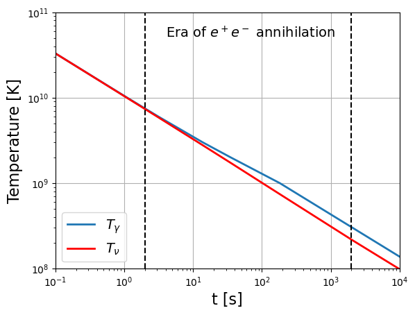
Figure 8:Temperature evolution of photons and neutrinos during annihilation (figure adapted from Weinberg (1989) p. 529,540 and originally from Peebles (1966)).
We can deduce the neutrino density as a function of . Neutrinos are fermions with 3 flavours, so if we assume that they have no mass, their density today would be :
which gives per flavour ( in total). For the energy density of the neutrino background, we find :
and numerically we find . From this we can deduce the total proportion of relativistic matter in the Universe (if neutrinos are relativistic):
The decoupling of the neutrinos was slightly superimposed on the annihilation of . As the neutrinos were still interacting at the time of annihilation, the neutrino background was slightly affected by the energy and entropy released by the annihilation of .In the literature, this is taken into account by introducing an effective number of neutrinos , numerically evaluated at 3.046. Taking this into account, the number of neutrinos and the energy density are :
Finally, the correct values and after annihilation are :
In fact, neutrinos have masses, with two important consequences (1) we do not know whether they are still relativistic today (all flavours taken together) (2) is greater than the value quoted above. Experiments observing neutrino oscillations dictate that the sum of neutrino masses, noted is greater than so at least one neutrino flavour would be non-relativistic today if compared to . From a cosmological point of view, if we very conservatively impose that then we end up with a constraint , and cosmological surveys looking at the gravitational collapse of the Universe’s Large-scale structures impose (DESI Collaboration et al. (2024)).
Big Bang Nucleosynthesis (BBN)
Let’s go back to about ms after the Big Bang, when the temperature of the Universe is a few tens of MeV. The Universe is then essentially a hot plasma in thermodynamic equilibrium composed of baryons, photons, electrons, positrons and neutrinos (about to decouple from the other particles). We recall that the baryon-to-photon ratio is a constant (18) and is more precisely:
with the measurement of from the power spectrum of CMB temperature anisotropies Planck Collaboration et al. (2020). As the Universe continues to expand, it cools down and protons and neutrons can fuse to form the first atomic nuclei. This is what we call Big Bang nucleosynthesis (BBN).
Neutron to proton ratio
The rate of formation of these nuclei will depend on an essential parameter: the ratio of the number of neutrons and protons available at the moment when the formation of nuclei becomes possible.
At ms, the protons and neutrons are in thermodynamic equilibrium with each other via the interactions :
and even this one (less effective):
As long as these interactions exist, the neutron to proton ratio is given by the equilibrium particle densities (55) for non-relativistic particles[6] :
Now . Moreover, according to the first reaction, at chemical equilibrium we have , so we can assume that if the chemical potentials of electrons and neutrinos are negligible. We deduce that the neutron to proton ratio is simplified to:
Consequently, as long as the temperature is such that , then there are as many neutrons as protons in the Universe. But below , the proportion of neutrons falls exponentially. Let be the ratio of neutrons to baryons if the species are in equilibrium at temperature . Then:
So the neutron density should be almost zero today, but this equation is only valid as long as the reactions are taking place. Indeed, if the expansion rate of the Universe becomes comparable to or greater than the interaction rate, then the reactions stop and the ratio is frozen at the value reached. The freeze mechanism of reactions involving massive particles is important in cosmology to understand the abundance of massive particles today.
For the reaction , the interaction rate is given by (Kolb & Turner (1990) p.90, Weinberg (1989) p.547 and originally in Peebles (1966)):
with the Fermi-Dirac distributions of the particles and :
with the Fermi constant and the axial-vector coupling of nucleons (Kolb & Turner (1990) p.91). Unfortunately, the 6 integrals giving the rates of the 6 reactions must be calculated numerically, because we will see that the neutron proportion freezes at a temperature close to and , which prevents us from making crude approximations to concentrate on a high or low energy regime.
Numerical approximation of integrals
A numerical approximation of the sum of the integrals for the two reaction interaction rates (117) is Bernstein et al. (1989) :
Next, to obtain the evolution of the neutron density, a numerical integration method is proposed in Dodelson (2003) p.67 by defining the neutron proportion :
To determine the freeze temperature of the ratio, we need to compare the reaction rates with the expansion rate . Let be the cumulative rate of the 3 interactions forming neutrons, and the sum of the other reactions forming protons. After numerical integration, we observe Figure 9 that decreases as a function of temperature and converges towards a plateau corresponding to the inverse of the neutron half-life time (independent of expansion). It is greater than the rate so it is the one that counts in the freeze mechanism. The rate is comparable to the expansion rate at the temperature:
This is the freeze temperature of the proportion of free neutrons. It occurs only after the Big Bang, so a short time compared to the half-life of the free neutron . We also note that , so no reasonable approximation could be made to calculate the integrals.
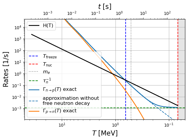
Figure 9:Comparison of the reaction rate and the expansion rate . The neutron density freeze temperature is defined by the intersection of the curves. The reaction rate reaches a plateau corresponding to the neutron decay rate, independent of expansion. The shaded region corresponds to the formation of atomic nuclei: there are no more free neutrons at this stage so the curves are no longer valid.
A detailed assessment of the neutron density allows us to write the following Boltzmann equation:
The last term of the equations corresponds to the dilution of particles with expansion if their number is conserved in a comoving volume. On the other hand, the total number of protons and neutrons is conserved in a comoving volume:
Let’s define the proportion of neutrons . The proportion of protons is deduced by . The differential equation for the neutron density is rewritten:
that is:
Let’s now study the relative neutron density . After numerical integration with the initial condition:
we obtain Figure 10. If the spontaneous decay of the neutron is omitted (dashed curve), the neutron fraction converges to , that is:
i.e. 1 neutron for 6 protons[7].
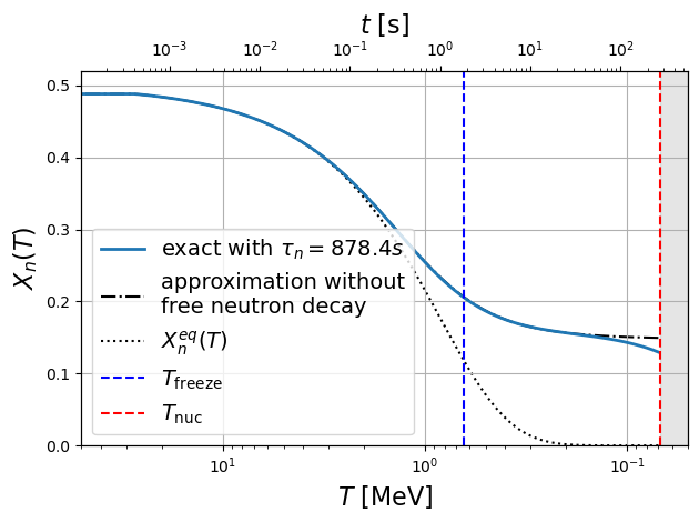
Figure 10:Neutron fraction as a function of time calculated by equation (130) (solid line). If neutron decay is neglected, then we obtain the dotted curve (). The equilibrium distribution gives the proportion of neutrons if the reactions are not frozen by the expansion of the Universe.
Synthesis of deuterium
After the neutron freeze temperature , the proportion of neutrons and protons is therefore stable, except that free neutrons have a half-life of about 15 minutes. However, if the temperature drops sufficiently, protons and neutrons can combine to form the lightest atomic nucleus by strong interaction, deuterium , via the reaction:
The question is therefore: when does the formation of deuterium take place and how many neutrons are available at that moment?
Deuterium has a binding energy:
It is therefore more favourable to form deuterium atoms than to keep protons and neutrons separate since . Note that this energy is higher than . However, we must remember that there are 109 photons per baryon and that these photons follow a blackbody distribution: even at energies comparable to , there is still a plethora of photons capable of dissociating the newly formed deuterium nuclei. The temperature of deuterium formation in the primordial universe must therefore necessarily involve , and will occur at a temperature lower than , when there are no longer enough very high energy photons capable of dissociating the nuclei.
Let’s calculate this temperature . We define the starting temperature of nucleosynthesis as that where half of the neutrons have been consumed to form deuterium, i.e. when . The ratio of particle densities at equilibrium is:
with (because deuterium is a massive spin 1 boson), , and (Ryden (2017) p.219).
The deuterium to neutron ratio is written:
Assuming that in any case the number of protons will decrease very little during the formation of deuterium, we can estimate that the proton density at is approximately:
We then deduce the temperature by the numerical inversion of the following equation, involving :
or s after the Big Bang, with from now on since the Universe has a temperature lower than . We note that is only slightly smaller than so the spontaneous decay of the free neutron must have lowered the proportion of neutrons available after . At , the fraction of neutrons still present is approximately:
The spontaneous decay of the neutron is therefore significant on this time scale.
Helium-4 synthesis
The formation of helium nuclei is only possible via the fusion of deuterium nuclei:
because it is much more unlikely that two protons and two neutrons would meet by chance to form a helium nucleus. However, the binding energy of helium 4 is much higher than that of deuterium ()[8], so its formation is highly favoured. Consequently, as soon as deuterium nuclei are available, they are almost immediately and totally fused into helium 4 nuclei and there are no longer any high-energy photons capable of dissociating them. Almost all the neutrons available at will therefore end up in a helium nucleus.
As two neutrons go into a helium-4 nucleus, the maximum number of formable helium nuclei is equal to half of the available neutrons (whether free or in deuterium nuclei). The helium-4 abundance in number of nuclei is deduced as:
In terms of mass, the abundance of helium 4 in the Universe at the end of primordial nucleosynthesis may be at most (Figure 11):
the remainder being hydrogen (at by mass). In terms of particle densities, we also obtain .
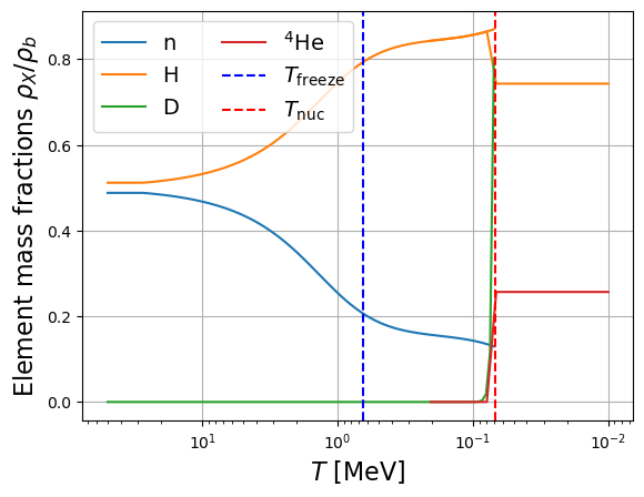
Figure 11:Mass fraction of the various light nuclei in the Universe over time, calculated using the simple model detailed in this chapter.
More precise calculations show that the synthesis of atomic nuclei starts about 3 minutes after the Big Bang and ends 20 minutes later. They predict around 24%, because a small fraction of neutrons remain in other light nuclei after such as deuterium, lithium, etc (Figure 12). These predictions are in good agreement with measurements (see Figure 13). Before the discovery of CMB temperature anisotropies in the 2000s, comparing measurements of light element abundances (by observing the interstellar medium or galaxies: horizontal grey bands in Figure 13) with these predictions was a way to measure and therefore (see equation (113)). The measurement of by temperature anisotropies (vertical grey band in Figure 13) is more precise but in agreement with BBN predictions, which shows the robustness of the standard model of cosmology (except for lithium where a disagreement persists).
In any case, with only the stellar mechanism of fusion of hydrogen at the core of stars into helium (and then fusion of helium into carbon, oxygen, etc), it is not possible to explain such an abundance of helium in the Universe. Only passing through a hot plasma at hundreds of millions of degrees containing free neutrons, even for at most 20 minutes while cooling, can explain the of helium present in the Universe. This is therefore important evidence for the existence of a state where the Universe was a hot, dense plasma for at least a few minutes.
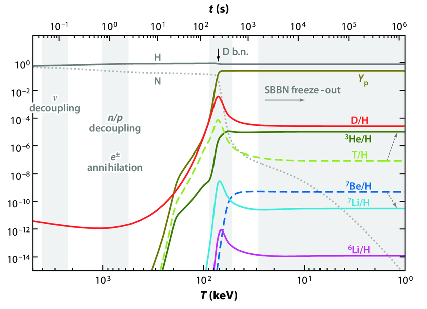
Figure 12:Synthesis of light elements in the primordial Universe (from Pospelov & Pradler (2010)).
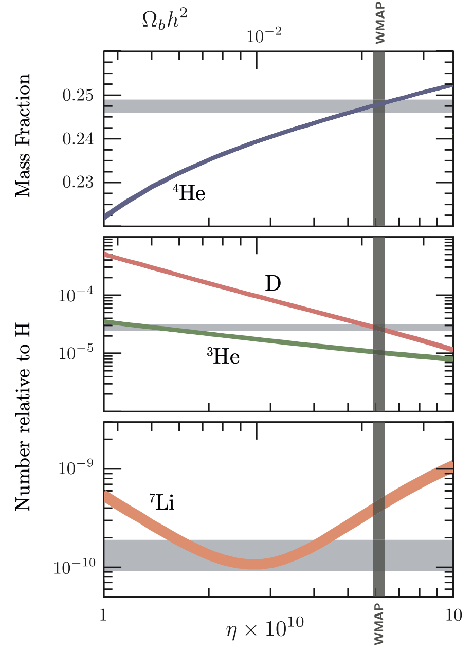
Figure 13:Comparison between theoretical predictions for the abundances of light nuclei (coloured bands) and measurements (grey bands) (from Baumann (2022)).
Recombination
In the primordial universe, recombination consists of two stages. First there is the formation of hydrogen atoms, then the decoupling of the remaining free electrons and photons. At this point, the plasma is transformed into a neutral gas of hydrogen and helium (plus a little lithium, etc.). After recombination, the photons in the thermal bath are free to propagate in the Universe since the medium is (almost) neutral. This first light corresponds to the cosmic microwave background and tells us about the state of the young Universe and the physics that took place there before (and after).
Formation of hydrogen atoms
The formation of hydrogen atoms proceeds by the reaction:
and we recall that the binding energy of hydrogen is . A quick approximation would give us that the temperature at which recombination took place is , but this would be forgetting that with a billion photons per baryon, even at lower temperatures the Universe still contains an enormous number of photons with energies high enough to ionize hydrogen atoms (the tail of the blackbody distribution). What we need to find, therefore, is the temperature for which the integral of the blackbody distribution at energies greater than gives a photon density comparable to . The parameter is therefore an important parameter that must be involved in estimating the temperature at recombination.
A better estimate must therefore be based at least on the baryon-to-photon ratio and . As for the abundance of deuterium, at equilibrium we can write:
with [9] and . This is Saha’s equation. Let be the fraction of free electrons in the primordial plasma:
By arguments of electrical neutrality and conservation of the number of particles, we also have:
assuming there is only hydrogen to simplify the calculations (we do not consider the recombination of helium[10]). Consequently, we have:
and simply:
therefore:
We have a second-degree equation in , involving , whose solution is (Ryden (2017) p.192):
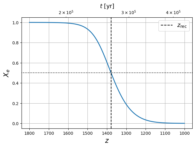
We define the moment of recombination as that when the medium is half ionized, i.e. or . Then the decoupling temperature is given by Ryden, 2017:
i.e. when the Universe is years old and its evolution is now dominated by its matter content. From Figure 15, however, we see that recombination extends globally between redshift 1200 and 1600, which still corresponds to about years, so it is not an instantaneous process for us humans, but still fast compared to the age of the Universe.
Photon decoupling
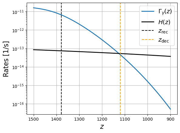
Figure 16:Comparison between the interaction rate and the expansion rate as a function of redshift.
For some time after , the photons remain coupled to the small fraction of free electrons by Thomson scattering:
The interaction rate is given by (see equation (21)) :
with the effective cross-section of Thomson scattering:
Decoupling occurs when this interaction rate becomes small compared to the expansion rate of the Universe (Figure 16), i.e.:
Since the Universe is then dominated by matter (), we have:
The result is:
By numerical resolution, we obtain:
Mean photon free path
Another way of looking at the decoupling of photons and matter, and therefore the moment when the Universe becomes transparent, is to look at the mean free path of photons . In the distant past, the Universe was opaque but the mean free path of photons could still be of the order of a few light-years. After decoupling, this becomes greater than the typical size of the Universe.
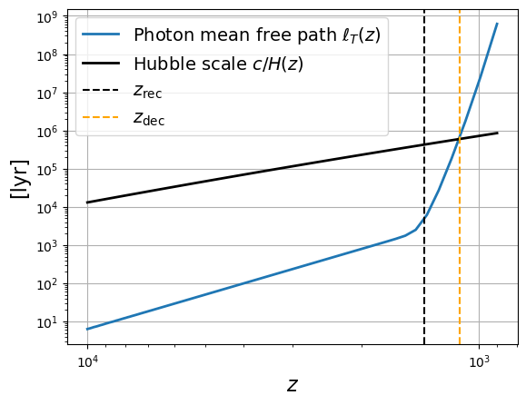
Figure 17:Comparison between the mean free path time of photons and the Hubble time .
The cosmic microwave background is therefore a blackbody radiation that was released about years after the Big Bang, when the Universe was almost no longer ionized since .
hadrons are divided into two families: mesons (2 quarks) and baryons (3 quarks). among the baryons, only protons are stable. The neutrons bound in atomic nuclei are stable, but when free they disintegrate into a proton with a half-life of 15 minutes. Mesons are all unstable with half-lives shorter than s. Electrons are 2000 times lighter than protons. Most of the mass of so-called ‘ordinary’ matter is therefore contained in atomic nuclei, hence the shorthand ‘baryonic matter’.
the classical limit appears for very low occupation numbers of energy levels, where the bosonic or fermionic nature of particles no longer matters since . It is valid at low density or high temperature, when the following condition is verified: , where is the average distance between particles and is the thermal de Broglie wavelength.
as early as 1ns after the Big Bang, the only surviving boson is the photon because the , and bosons decay. Moreover, when they appear during the electroweak transition around GeV, their masses are such that they are already too heavy to be relativistic. Therefore, only photons should be considered in the list of relativistic bosons, whose chemical potential is zero at thermodynamic equilibrium.
since electric charge is associated with Coulomb forces and the expansion of the Universe is governed only by gravitational forces, the Universe must be globally neutral.
strictly speaking an entropic integration constant must appear but this is zero by virtue of the third principle of thermodynamics.
we recall that the masses of protons and neutrons are about .
the helium 4 nucleus has a so-called magic number of neutrons and protons (Magic number (physics)) which stabilizes it and gives it a binding energy much higher than deuterium or lithium, its neighbors in the periodic table of elements.
a hydrogen atom can have a spin 0 (inverted spins) or 1 (aligned spins) so 4 internal degrees of freedom.
with one neutron for 7 protons, so in number more than of baryons are protons.
- Planck Collaboration, Aghanim, N., Akrami, Y., Ashdown, M., Aumont, J., Baccigalupi, C., Ballardini, M., Banday, A. J., Barreiro, R. B., Bartolo, N., Basak, S., Battye, R., Benabed, K., Bernard, J.-P., Bersanelli, M., Bielewicz, P., Bock, J. J., Bond, J. R., Borrill, J., … Zonca, A. (2020). Planck 2018 results - VI. Cosmological parameters. A&A, 641, A6. 10.1051/0004-6361/201833910
- Rubin, V. C., & Ford, W. Kent, Jr. (1970). Rotation of the Andromeda Nebula from a Spectroscopic Survey of Emission Regions. The Astrophysical Journal, 159, 379. 10.1086/150317
- Alpher, R. A., & Herman, R. (1948). Evolution of the Universe. Nature, 162(4124), 774–775. 10.1038/162774b0
- Gamow, G. (1948). The Evolution of the Universe. Nature, 162(4122), 680–682. 10.1038/162680a0
- Penzias, A. A., & Wilson, R. W. (1965). A Measurement of Excess Antenna Temperature at 4080 Mc/s. The Astrophysical Journal, 142, 419. 10.1086/148307
- Penzias, A. A., & Wilson, R. W. (1965). Measurement of the Flux Density of CAS a at 4080 Mc/s. The Astrophysical Journal, 142, 1149. 10.1086/148384
- Fixsen, D. J. (2009). The temperature of the cosmic microwave background. The Astrophysical Journal, 707(2), 916–920. 10.1088/0004-637X/707/2/916
- Condon, J. J., & Matthews, A. M. (2018). ΛCDM Cosmology for Astronomers. Publications of the Astronomical Society of the Pacific, 130(989), 073001. 10.1088/1538-3873/aac1b2
- Mather, J. C., Fixsen, D. J., Shafer, R. A., Mosier, C., & Wilkinson, D. T. (1999). Calibrator Design for the COBE Far-Infrared Absolute Spectrophotometer (FIRAS). The Astrophysical Journal, 512(2), 511–520. 10.1086/306805
- Hurier, G., Aghanim, N., Douspis, M., & Pointecouteau, E. (2014). Measurement of theTCMBevolution from the Sunyaev-Zel’dovich effect. Astronomy & Astrophysics, 561, A143. 10.1051/0004-6361/201322632
- Noterdaeme, P., Petitjean, P., Srianand, R., Ledoux, C., & López, S. (2011). The evolution of the cosmic microwave background temperature: Measurements ofTCMBat high redshift from carbon monoxide excitation. Astronomy & Astrophysics, 526, L7. 10.1051/0004-6361/201016140
- Kolb, E. W., & Turner, M. S. (1990). The Early Universe (Vol. 69). 10.1201/9780429492860
- Weinberg, S. (1989). The cosmological constant problem. Reviews of Modern Physics, 61(1), 1–23. 10.1103/RevModPhys.61.1
- Nakamura, K., & others. (2010). Review of particle physics. Chapter 33: Statistics. J.Phys., G37, 075021. 10.1088/0954-3899/37/7A/075021
- Peebles, P. J. E. (1966). Primordial Helium Abundance and the Primordial Fireball. II. \apj, 146, 542. 10.1086/148918