Until now, we have studied the evolution of a homogeneous Universe, at least at very large scales, beyond approximately . However, today we observe that matter is agglomerated in the form of planets, stars, galaxies, galaxy clusters and superclusters of galaxies. The question that arises in this chapter is: how do these structures form in an expanding Universe? If the formation of the smallest objects involves many physical processes and is highly dependent on local initial conditions, it is possible to develop a simple linear model for the evolution of the largest structures , such as galaxy clusters or superclusters. To do this, we will simply use a Newtonian theory of linear perturbations, and calculate the evolution of these perturbations in an expanding Universe.

Figure 1:Size and mass scales in the Universe.
1Range of Validity
However, let us state the necessary conditions for the validity of the Newtonian perturbation theory. A first obvious condition is that the perturbation of the metric and of the energy-momentum tensor must be small. In the case of non-relativistic matter, this means that density perturbations must remain small compared to the average density i.e. . Perturbations of the gravitational field are also small compared to the average gravitational field i.e. .
But to be able to return to Newtonian gravity in a homogeneous expanding spacetime and study only density perturbations, there is another condition. The size of the studied regions must be much smaller than the Hubble radius , because in Newtonian gravitation the interaction propagates instantaneously. If the structure is of cosmological size, by the time the information from a collapsing region has traveled to its boundaries, the expansion factor changes significantly: a situation that obviously cannot be treated using Newtonian gravity. We therefore only consider structures of size much smaller than to be able to assume that the gravitational force propagates instantaneously in the structure with respect to the expansion rate of the Universe.
2Classical Acoustics Preamble
The non-relativistic matter field is described by a perfect fluid model. Looking at the evolution of perturbations in a perfect fluid means studying the field of acoustics. Let us recall some useful notions here.
In an Eulerian description of fluids, for a perfect fluid at rest, we define its velocity field , its pressure field and its mass density field as constants:
On top of this, we superimpose small amplitude perturbations:
The generated overpressures change the internal energy of the perturbations and thus their temperature, and this work of pressure forces allows the propagation of acoustic energy. In acoustics, we measure that compressions are adiabatic and reversible, meaning that the size of perturbations is larger than the mean free path of fluid particles: we can then neglect heat conduction. We therefore use the isentropic compressibility instead of the isothermal compressibility :
We deduce the link between pressure and density perturbations via the isentropic compressibility:
We also have local mass conservation:
Since the fluid is perfect, its dynamics is governed by the Euler equation (Navier-Stokes without viscosity):
where we usually neglect gravitation. By combining these three equations, we obtain a d’Alembert equation:
with the speed of sound.
For a perfect gas and isentropic transformations, we use Laplace’s Law with the ratio of heat capacities at constant pressure and constant volume , also called the adiabatic index. If the fluid particles possess degrees of freedom (translations, rotations, vibrations) to store energy in kinetic (thermal) form, then the adiabatic index is . For a diatomic gas like air at usual temperature, there are degrees of freedom (3 translations and 2 rotations) so . We deduce a formula for the speed of sound as a function of temperature and particle mass[1]:
with the molar mass of the fluid and the effective mass of an air particle if that is the medium considered, calculated by:
3Acoustics in Expanding Space with Gravitation
At the emission of the CMB, we observe that the Universe is a perfect gas of non-relativistic matter, slightly inhomogeneous, with density enhancements of reduced size (of the order of ). These fluctuations will a priori increase over time thanks to gravitational attraction, to result in a Universe where the density contrast is of the order of [2] ( Figure 1,Figure 2). What are the mechanisms allowing this growth?
The formation of large-scale structures in the Universe can be understood through a linear perturbation theory in the perfect fluid constituted by non-relativistic matter after recombination. To study the evolution of these density perturbations in the matter field, it is therefore a matter of rewriting the previous acoustic equations, in the particular context of an expanding medium subject to the laws of gravity.
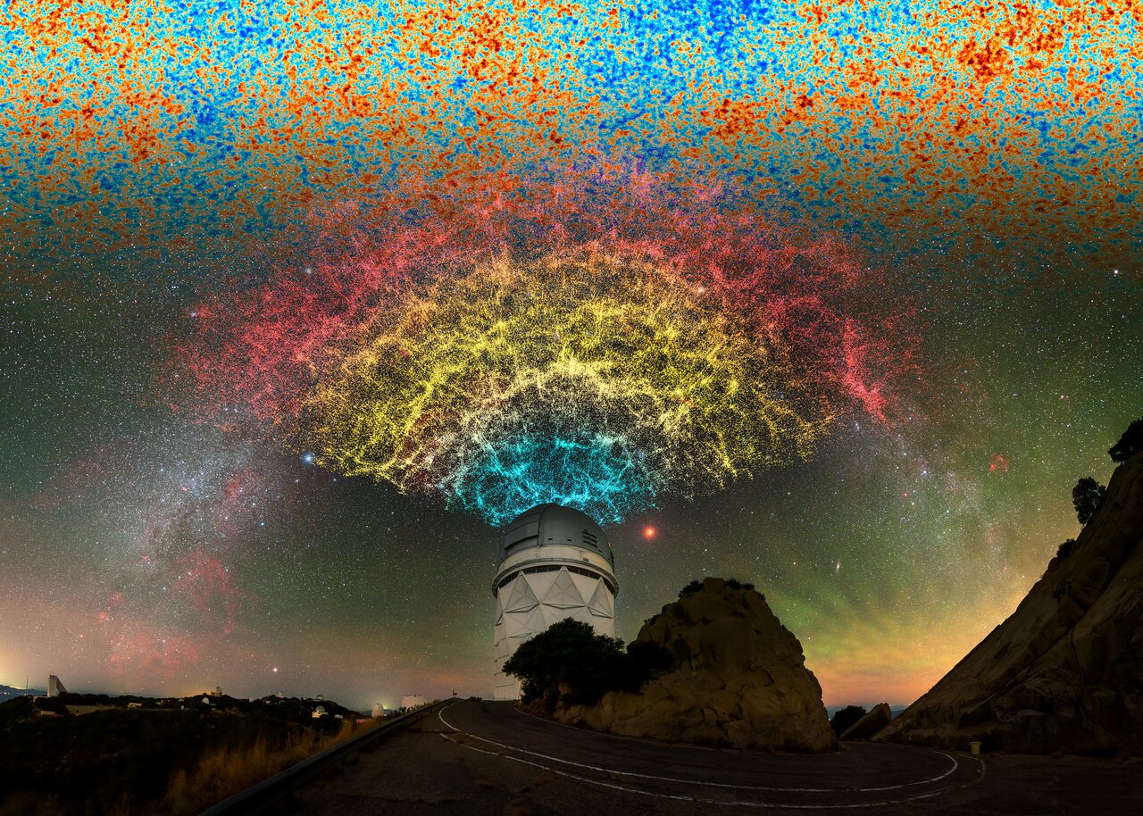
Figure 2:An artistic celebration of the Dark Energy Spectroscopic Instrument (DESI) Year 1 data, showing a slice of the larger 3D map that DESI is constructing during its five-year survey. DESI is mounted on the Nicholas U. Mayall 4-meter Telescope at Kitt Peak National Observatory. Credit: DESI Collaboration/KPNO/NOIRLab/NSF/AURA/P. Horálek/R. Proctor
Figure 3:This simulation shows how gravity affects the position of observed galaxies, thus modifying the way matter clumps together to form cosmic structures. As different gravity models predict different structure formations, DESI scientists can compare observations with predictions and thus test gravity at cosmological scales. Credit: Claire Lamman and Michael Rashkovetskyi / DESI collaboration
Coordinate Systems
The equations of classical physics are valid using physical (non-comoving) quantities: proper distance, proper time, etc... The use of physical distances as a coordinate system is however impractical in an expanding Universe because time and distance are linked. A more practical method is to write these equations in comoving space. Let us denote:
the physical position vector (whose norm is the proper distance ),
the comoving position vector (whose norm is the comoving distance ),
the physical velocity,
the comoving velocity.
We have the following relations:
Although the Hubble flow (first term of (11)) should not be considered as a real velocity, it appears in the relationship between and . This would pose a problem if it could take values of the order of (or larger). But the condition that guarantees that (see section Section 1).
How do we switch from the physical coordinate system to the comoving coordinate system? The conversion of spatial partial derivatives is quite simple:
The time partial derivative requires more careful examination. Let us write the differential of any function of time and space :
Therefore by identification:
Mass Conservation
In physical space, the continuity equation is written:
Using the comoving density , we can express this equation in comoving space:
By introducing the classical vector calculus formula
where is a scalar and a vector, the above equation reduces to:
The continuity equation therefore takes exactly the same form in comoving space, using comoving variables. However, this is not the case if we use the peculiar velocity .
Euler Equation
In physical space, the Euler equation for a self-gravitating perfect (non-viscous) fluid takes the usual form:
In comoving space, it transforms into:
with the comoving potential. Ensuring that:
the Euler equation in comoving coordinates reduces to:
We can see two additional terms compared to the version of the Euler equation written in physical coordinates. The additional term is a drag force created by the expansion on comoving velocities. The last term depends only on kinematic quantities, so it is a fictitious force linked to the change of coordinate system, non-zero if and only if there is acceleration between the reference frames (). In an accelerating expanding universe (), it corresponds to a centripetal fictitious force.
Poisson Equation
In a universe without cosmological constant, from general relativity we deduce the usual Poisson equation in the weak field limit (38):
where is the gravitational potential. Given the relationship between the potential and the Newtonian force, the comoving potential is naturally defined as , and the Poisson equation is also unchanged in comoving space:
4Newtonian Theory of Perturbations
Zeroth Order Solution
In a homogeneous and isotropic universe, at zeroth order the mass density does not depend on space and matter is globally at rest. There is therefore no global peculiar velocity and the mass conservation equation in comoving space (18) admits the zeroth order solution:
The comoving mass density therefore remains stationary and homogeneous. The integration of the Poisson equation (24) in spherical coordinates[3] gives:
If we use the Friedmann equations (60):
for a matter-dominated Universe with and , we obtain the force derived from the gravitational potential:
The gradient of the gravitational field gives at zeroth order a centrifugal force reflecting the repulsive character of the universe’s expansion.
From the Euler equation (22) and the previous results, we logically arrive at finding that therefore:
consistent with a homogeneous Universe.
First Order Linear Solution
Let us consider small perturbations around the zeroth order solution:
The quantity is called the density contrast and is widely used in structure formation theory. Note that it has the same value in physical space and in comoving space. By injecting these expressions into the continuity, Poisson and Euler equations, the zeroth order solution disappears (as expected) and by removing second order terms, we obtain the set of linearized equations:
By taking the divergence of the linearized Euler equation (34), the time derivative of the linearized mass conservation equation (33) and reinjecting the Poisson equation (35), we finally obtain:
We introduce the speed of sound in the medium for adiabatic compressions:
Then we obtain the perturbation growth equation in comoving space:
Let us compare this equation to the d’Alembert equation obtained in classical acoustics (7). We have two additional terms:
a friction term which will slow down structure formation all the more as the expansion rate is high, on cosmological time scales ;
a source term proportional to which models gravitational collapse (the more marked the structure, the more it collapses). The evolution of matter perturbations is therefore dictated by the relative intensities of the gravitational force (attractive), pressure forces (repulsive), and the expansion of the Universe (damping).
Speed of Sound
In a radiation-dominated Universe, the properties of the relativistic gas are:
hence the speed of sound in the relativistic plasma:
Just before recombination, the propagation of sound waves is therefore relativistic in the primordial plasma.
In a non-relativistic matter-dominated Universe, the thermodynamic properties of baryons are:
with the effective mass of baryons in a mixture of atomic hydrogen and helium gas (note the resemblance with (10)), and the adiabatic index of baryons because hydrogen is in atomic form (and helium of course). For a reversible adiabatic transformation, with Laplace’s law we have , the baryon temperature evolves as:
But so the baryon temperature evolves as:
With , for baryons the pressure varies as and the temperature as . The speed of sound in the baryon gas is written:
Just after photon-electron decoupling, the baryon temperature is so the speed of sound in the baryon gas is approximately . Around recombination, the change is of several orders of magnitude so the evolution of perturbations changes drastically at this moment. Then the baryon temperature decreases as , at least as long as heating by interstellar radiation does not change things (around ). The speed of sound therefore decreases as in our linear model.
/Users/jneveu/miniforge3/envs/m2-cosmo/lib/python3.11/site-packages/astropy/cosmology/flrw/base.py:1072: IntegrationWarning: The integral is probably divergent, or slowly convergent.
  return quad(self._lookback_time_integrand_scalar, z, inf)[0]
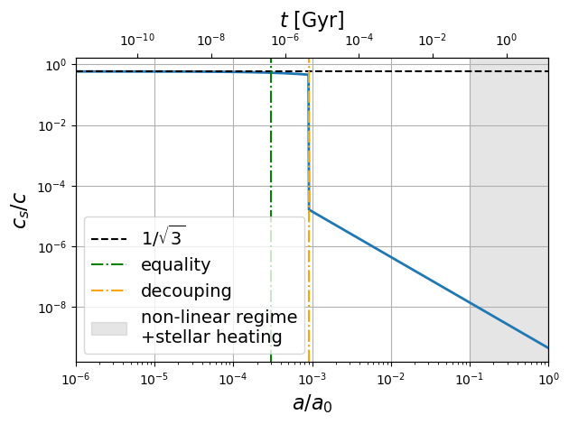
Figure 4:Speed of sound in the Universe as a function of the scale factor . The slight decrease between equivalence and decoupling is given by equation (48) (see box). The calculation is inaccurate when we enter the non-linear regime of structure growth i.e. when (shaded region). Moreover, around this redshift also, the baryon gas is heated by stellar radiation so the baryon temperature no longer evolves as .
Mixture of Baryons and Coupled Photons
As long as photons are coupled to free electrons, they are mechanically coupled to the baryon gas by the Coulomb force. During the period when the Universe is dominated by matter but photons are still coupled to electrons (Weinberg (1989) p.509,566):
Jeans Instability
The solutions to the perturbation evolution equation (38) will be studied in the next semester, but we can already study their behavior from their dispersion relation. Let us look for plane wave solutions of the form:
and study the solutions in Fourier domain. The dispersion relation is written:
By neglecting the damping term (of the order of the age of the Universe) compared to the characteristic time of perturbation evolution (), we arrive at:
with . This is the same dispersion relation as that of electromagnetic waves in a plasma. We define the Jeans wavenumber (The Royal Society (1902)) and the Jeans length by:
If , then so we have an oscillating solution i.e. an acoustic wave that propagates: perturbations of size small compared to the Jeans length oscillate thanks to the pressure force and do not grow.
If , so we have a non-oscillating exponential solution: large structures evolve only under the effect of gravity and grow (and voids decrease).
Since the scale evolves with expansion () as well as the Jeans length, the discussion is not easy to conduct along the history of the Universe. Let us define the mass in a sphere of radius , conserved with expansion, and compare it to the Jeans mass :
We now have only one quantity that varies with :
If , then the structure is too light and pressure can compensate for the force of gravity: the structure oscillates.
If , then the structure is too heavy and collapses gravitationally.
The plot of the Jeans mass as a function of the scale factor allows us to predict which structures can collapse gravitationally and those whose growth is prevented Figure 5 (Weinberg (1989) p. 565).
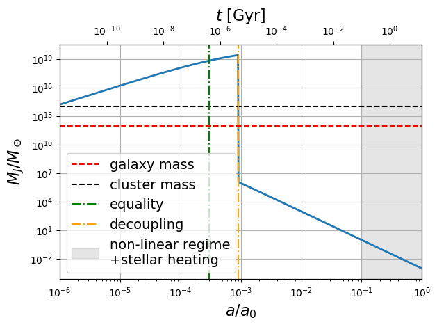
Figure 5:Evolution of the Jeans mass as a function of the scale factor . The calculation is inaccurate when we enter the non-linear regime of structure growth i.e. when (shaded region). Moreover, around this redshift also, the baryon gas is heated by stellar radiation so the baryon temperature no longer evolves as .
Describing structure growth before recombination contradicts the non-relativistic hypothesis on which our study is based. However, the speed of sound scale remains a relevant scale and moreover non-relativistic matter dominates after equivalence. Knowing this (and that the relativistic study does not give fundamentally different results from what follows), we will allow ourselves to discuss the growth of large structures in the primordial and recent Universe (although it is non-linear today).
According to Figure 5, we see that before decoupling structures with the mass of a galaxy or galaxy cluster are not heavy enough to collapse (or only in the very first moments of the Universe). Pressure waves travel through them and they oscillate. However, after decoupling, the speed of sound drops by 5 orders of magnitude. The decoupling of photons freezes the pressure waves and structures with the mass of galaxies and even dwarf galaxies can begin their growth.
Statistical Description of Perturbations
Gaussian Field
Let us describe the field in Fourier space. We use the following convention for direct and inverse Fourier transforms:
The field in Fourier is a complex number described by its modulus and phase which we will denote:
At the moment of the Big Bang, we can think that the phases are randomly and independently distributed (no coupling between scales , see chapter ). If perturbations follow a linear evolution, then the modes evolve independently of each other: the phases remain independent random variables. But if the phases of a field in Fourier are random and independent, then this field is called a Gaussian field. If we examine the inverse Fourier transform, we note indeed that the field in real space is the result of the sum of independent random variables so we can apply the central limit theorem: the result of the sum follows a Gaussian distribution. This field is therefore statistically entirely defined by the two parameters of the Gaussian distribution, its mean and its variance:
with since this field is physical hence real (). Strictly speaking, the notation designates an average over a statistical ensemble of realizations. However, since we only have one realization of the universe, this will be an average over a volume with samples of . The mean is zero by definition of the density contrast, so let us focus on the variance.
Matter Power Spectrum
The conjugate of a Fourier mode is written:
so the variance can be rewritten:
For an isotropic field, only the norm of the vector matters therefore:
We define the matter power spectrum by:
where denotes here the Dirac delta function, homogeneous to the inverse of a volume. In the sense of distributions, its Fourier transform equals 1 which allows us to deduce a formulation in the form of an integral:
The power spectrum is therefore homogeneous to a volume: . For a real field, the conjugate Fourier modes verify so we can resume the definition of the power spectrum and calculate the mean of the norm of the Fourier modes:
with an integration volume, in practice finite because measurements or simulations are discrete and realized in a finite volume. For an isotropic field, we can perform the ensemble average by averaging over modes of same norm . We obtain:
The matter power spectrum at a scale is therefore the average of Fourier modes of same norm. We also define the modal logarithmic variance as:
This is the contribution to the variance of modes of norm per logarithmic interval:
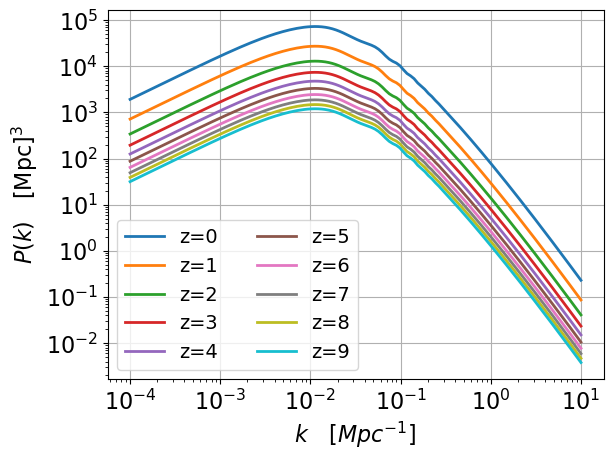
In the context of linear structure growth, Fourier modes are independent. The matter power spectrum at a redshift can then be written:
where we define the transfer function and the initial matter power spectrum . What could it be? If we assume that at the beginning of the Universe density perturbations are random and there is no particular distance scale, a power law is appropriate:
For initial conditions, we will prefer to focus on scalar perturbations of the metric . But by Poisson’s equation . We deduce the normalized power spectrum of scalar fluctuations:
In the early 1970s, cosmologists Harrison and Zel’dovich proposed that all scales should contribute equally to the variance at the beginning of the Universe, no spatial scale counts more than others (Harrison (1970), Zeldovich (1972)). If this hypothesis is true, then we must have .
The theoretical prediction of the spectrum by looking at the evolution of different density perturbation scales along the history of the Universe is a convex curve, presenting a form in at large scales (too large to have evolved) and in at small scales (those that collapse). The switch between the two regimes is the mode corresponding to the horizon scale at equivalence (see Figure 6).

Figure 6:Matter power spectrum measured by different techniques and compared with theoretical linear (solid line) and non-linear (dotted line) predictions, adapted from Chabanier et al. (2019).
Correlation Function and 
The power spectrum is related to the correlation function in physical space by the following formulas:
We note that autocorrelation gives back the variance of the field: , and that the latter corresponds roughly to the integral of the matter power spectrum hence to its normalization. The measurement of the power spectrum normalization is therefore a way to measure matter clumping: the higher the power spectrum, the higher the variance of the matter field, hence the more matter is condensed into overdensities. From an experimental point of view, the power spectrum is measured by galaxy counting in spheres of radius :
Today, Tristram, M. et al. (2024) measures:
Since this value is close to 1, this means that at scales smaller than we are already in a non-linear regime of structure growth since . Intuitively, we also understand that since structures collapse gravitationally over time, the variance of the matter field increases hence the normalization of also (Figure 7).
Acoustic Waves in the Primordial Universe
Before decoupling, acoustic waves travel through the primordial plasma. Let us define the comoving sound horizon as:
the maximum comoving distance traveled by an acoustic wave since the beginning of the Universe. At the moment of decoupling, it is worth or . This is therefore the distance that a wave from an overdensity present at the Big Bang could travel. This wave propagation translates into a positive correlation on the presence of matter at this fundamental spatial scale. This scale converts into an angular separation on the sky, imprinted on the CMB temperature anisotropy map and given by:
A scale in distance space gives a sinusoidal power spectrum in reciprocal space. Measuring the position of maxima in the CMB temperature anisotropy power spectrum leads to a precise measurement of the sound horizon Tristram, M. et al., 2024:
Measuring the amplitude of the spectrum as well as the slope at large scales (small of Figure 10) allows to trace back to the parameters of the initial power spectrum:
We note that is close to 1, confirming the initial intuition of the Harrison-Zel’dovich spectrum. The fact that is slightly less than 1 (at more than 5\sigma) is a signature of inflation models (see next chapter). Finally, the fact that the second peak is attenuated compared to the first and third peak is a signature of the presence of baryons, which allows to measure:
Figure 8:Time evolution of 10 Gaussian peaks under the effect of acoustic propagation.
Figure 9:Time evolution of a Gaussian field with an initial power spectrum . Left, the evolution of the map. Center, the stacking of 1000 thumbnails centered on initial peaks. Right, the evolution of the power spectrum.
Figure 10:Power spectrum of CMB temperature fluctuations as a function of angular mode Tristram, M. et al., 2024.
:name: fig:desi_peaks :align: center :width: 60%
Illustration of BAO formation in galaxy distribution. Credit: DESI collaboration
Adiabatic or Isocurvature Initial Conditions?
Initial fluctuations can be either adiabatic or isocurvature. In the adiabatic case, we have equality of fluctuations for all components of the Universe: , and we predict the presence of all harmonics (1,2,3,...) in the CMB power spectrum. In the isocurvature case, the total density fluctuation is zero so we have oppositions like . We then predict the presence of only odd peaks in the CMB spectrum (1,3,5,...). The presence of all peaks indicates that initial conditions were adiabatic (Hu & Sugiyama (1995) p. 27).
Can We See the CMB Evolve Over Time?
To be reworked: https://
On what time scale should we then expect to see the CMB change? The smallest scales we can currently resolve are about in the sky, which corresponds to about \num{50 000} light-years (15\,\kpc) at the distance of the CMB.
For a structure of \num{50 000} light-years, the light from the far end takes \num{50 000} years longer to reach us than light from the near end. Does this mean we should expect CMB temperature fluctuations at these scales to change in about \num{50 000} years? Well, not quite. The CMB is redshifted by a factor of 1100, which means its apparent evolution in time is dilated by the same factor. We therefore expect fluctuations at the (currently) smallest resolved scales to change on a time scale (1100 times longer) of about 55 million years.
Optical Depth
We define the optical depth by the ratio of the number of photons received on Earth without having undergone any Thomson scattering to the number of photons emitted at a time :
with
The time for which is called the time of last scattering. This is the time since which a CMB photon has not interacted with an electron. More precisely,
This is one of the six parameters of the standard CDM model. Indeed, after the emission of the cosmic microwave background, we enter the Dark Ages of the Universe, when the Universe is transparent but no stars are yet emitting light. But with the birth of the first stars and galaxies, perhaps 150 million years after the Big Bang, the neutral medium is ionized once again. Although very sparse, CMB photons again interact with electrons by Thomson scattering, which reduces the amplitude of small-scale anisotropies in the CMB power spectrum, and introduces new anisotropies in polarization anisotropies. This is the least well measured parameter of the CDM model at the moment (Figure 12) Tristram, M. et al., 2024, but it informs about the appearance of the first luminous objects (Figure 13).
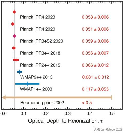
Figure 12:The optical depth to reionization measured as a smearing of the CMB angular power spectrum (from https://
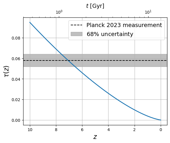
Figure 13:Assuming that the Universe is once again completely ionized, the calculation of its optical depth shows that if today we measure then the reionization of the Universe should be complete around giving the start of galaxy formation earlier than 1 billion years after the Big Bang.
- Einstein, A. (1917). Kosmologische Betrachtungen zur allgemeinen Relativitätstheorie. Sitzungsberichte Der Königlich Preussischen Akademie Der Wissenschaften, 142–152. https://adsabs.harvard.edu/pdf/1917SPAW.......142E
- Weinberg, S. (1989). The cosmological constant problem. Reviews of Modern Physics, 61(1), 1–23. 10.1103/RevModPhys.61.1
- (1902). Philosophical Transactions of the Royal Society of London. Series A, Containing Papers of a Mathematical or Physical Character, 199(312–320), 1–53. 10.1098/rsta.1902.0012
- Harrison, E. R. (1970). Fluctuations at the Threshold of Classical Cosmology. Physical Review D, 1(10), 2726–2730. 10.1103/physrevd.1.2726
- Zeldovich, Y. B. (1972). A Hypothesis, Unifying the Structure and the Entropy of the Universe. Monthly Notices of the Royal Astronomical Society, 160(1), 1P-3P. 10.1093/mnras/160.1.1p
- Chabanier, S., Millea, M., & Palanque-Delabrouille, N. (2019). Matter power spectrum: from Ly α forest to CMB scales. Monthly Notices of the Royal Astronomical Society, 489(2), 2247–2253. 10.1093/mnras/stz2310
- Tristram, M., Banday, A. J., Douspis, M., Garrido, X., Górski, K. M., Henrot-Versillé, S., Hergt, L. T., Ilić, S., Keskitalo, R., Lagache, G., Lawrence, C. R., Partridge, B., & Scott, D. (2024). Cosmological parameters derived from the final Planck data release (PR4). A&A, 682, A37. 10.1051/0004-6361/202348015
- Hu, W., & Sugiyama, N. (1995). Toward understanding CMB anisotropies and their implications. Physical Review D, 51(6), 2599–2630. 10.1103/physrevd.51.2599