Cosmological models Université Paris-Saclay
IJCLab
1 Simple models ¶ Now that we have a model to describe the dynamics of the Universe, let’s calculate its evolution in a few simple cases for practice.
Flat universe, matter only ¶ Let’s start with the case of a flat Universe containing only non-relativistic matter. This is the so-called Einstein-de Sitter model. It is the simplest one could think of in 1930. The first Friedmann equation is written:
3 a ˙ 2 a 2 = 8 π G ρ m = 8 π G ρ m 0 ( a 0 a ) 3 ⇔ ( a ˙ ) 2 = 8 π G ρ m 0 a 0 3 / 3 a = H 0 2 Ω m 0 a 0 3 a \begin{align*}
& 3 \frac{\dot{a}^2}{a^2} = 8\pi \GN \rho_m = 8 \pi \GN \rho_m^0 \left(\frac{a_0}{a}\right)^{3}
& \Leftrightarrow (\dot a)^2 = 8 \pi \GN \rho_m^0 a_0^3 / 3 a = H_0^2 \Omega_m^0 \frac{a_0^3}{a}
\end{align*} 3 a 2 a ˙ 2 = 8 π G ρ m = 8 π G ρ m 0 ( a a 0 ) 3 ⇔ ( a ˙ ) 2 = 8 π G ρ m 0 a 0 3 /3 a = H 0 2 Ω m 0 a a 0 3 Before integrating this differential equation, let us remember that the energy density parameters are linked by a closure relation (94) Ω m 0 = 1 \Omega_m^0=1 Ω m 0 = 1 a a a
∫ 0 a a ′ a 0 d a ′ a 0 = ∫ 0 t H 0 d t ′ ⇒ 2 3 ( a ( t ) a 0 ) 3 / 2 = H 0 t \int_0^{a}\sqrt{\frac{a'}{a_0}} \frac{\dd a'}{a_0} = \int_0^t H_0 \dd t' \Rightarrow \frac{2}{3}\left(\frac{a(t)}{a_0}\right)^{3/2} = H_0 t ∫ 0 a a 0 a ′ a 0 d a ′ = ∫ 0 t H 0 d t ′ ⇒ 3 2 ( a 0 a ( t ) ) 3/2 = H 0 t ⇒ a ( t ) a 0 = ( 3 2 H 0 t ) 2 / 3 \Rightarrow \frac{a(t)}{a_0} = \left( \frac{3}{2}H_0 t\right)^{2/3} ⇒ a 0 a ( t ) = ( 2 3 H 0 t ) 2/3 with at the beginning of the Universe t = 0 t=0 t = 0 a = 0 a=0 a = 0
Flat universe, radiation only ¶ By similar reasoning, we show that for a flat Universe dominated by radiation we have a different evolution of the scale factor:
a ( t ) a 0 = ( 2 H 0 t ) 1 / 2 \frac{a(t)}{a_0} = \left( 2 H_0 t\right)^{1/2} a 0 a ( t ) = ( 2 H 0 t ) 1/2 Empty universe (Milne) ¶ Suppose that the Universe is empty, or at least with a total energy density much lower than the critical density. Then the Universe must be curved since in this case:
Ω k 0 = 1 − Ω m 0 − Ω r 0 − Ω Λ 0 ≈ 1 \Omega_k^0 = 1 - \Omega_m^0 - \Omega_r^0 - \Omega_\Lambda^0 \approx 1 Ω k 0 = 1 − Ω m 0 − Ω r 0 − Ω Λ 0 ≈ 1 This Universe is therefore hyperbolic[1]
a ˙ 2 a 2 = H 0 2 Ω k 0 a 0 2 a 2 = H 0 2 a 0 2 a 2 \frac{\dot{a}^2}{a^2} = H_0^2 \Omega_k^0 \frac{a_0^2}{a^2} = H_0^2 \frac{a_0^2}{a^2} a 2 a ˙ 2 = H 0 2 Ω k 0 a 2 a 0 2 = H 0 2 a 2 a 0 2 then:
a ˙ = a 0 2 H 0 2 = a 0 H 0 \dot a = \sqrt{a_0^2 H_0^2} = a_0 H_0 a ˙ = a 0 2 H 0 2 = a 0 H 0 Integration therefore gives a Universe expanding at constant velocity:
a ( t ) = a 0 H 0 t a(t) = a_0 H_0 t a ( t ) = a 0 H 0 t The Hubble constant H 0 H_0 H 0 a ( t ) a(t) a ( t )
2 Multi-component models ¶ Modern cosmology was born with General Relativity. Since the writing of these equations, scientists have begun to mathematically describe the universe as a physical system. Many models have been proposed to describe the different histories of the universe.
Eddington-Lemaître model (1927) ¶ Friedmann and Lemaître were the first cosmologists to independently propose non-static universe models with arbitrary curvatures. Friedmann’s equations have been extensively studied in this course, but Lemaître was the first to propose the idea that the Universe developed from a primeval atom. His model is based on a universe composed only of cold matter, with a cosmological constant and arbitrary spatial curvature (no radiation).
In such a model, show that, just after a big bang at t = 0 t=0 t = 0
a ( t ) a 0 = ( 3 2 H 0 Ω m 0 t ) 2 / 3 \frac{a(t)}{a_0} =\left( \frac{3}{2}H_0\sqrt{\Omega_m^0}t\right)^{2/3} a 0 a ( t ) = ( 2 3 H 0 Ω m 0 t ) 2/3 As the universe expands, however, the energy density of matter decreases and the cosmological constant eventually dominates. Show that, for large t t t
a ( t ) ∝ e H 0 Ω Λ 0 t a(t) \propto e^{H_0\sqrt{\Omega_\Lambda^0}t} a ( t ) ∝ e H 0 Ω Λ 0 t Calculate a ¨ \ddot{a} a ¨ a ∗ a_* a ∗
In the Lemaître matter-only model, the first Friedmann equation is written:
a ˙ 2 a 2 = H 0 2 [ Ω m 0 ( a 0 a ) 3 + Ω Λ 0 + Ω k 0 ( a 0 a ) 2 ] ⇔ a ˙ 2 = H 0 2 [ Ω m 0 a 0 3 a + Ω Λ 0 a 2 + Ω k 0 a 0 2 ] \frac{\dot{a}^2}{a^2} = H_0^2\left[\Omega_m^0 \left(\frac{a_0}{a}\right)^{3} + \Omega_\Lambda^0 + \Omega_k^0 \left(\frac{a_0}{a}\right)^{2}\right] \Leftrightarrow \dot{a}^2 = H_0^2\left[\Omega_m^0 \frac{a_0^3}{a} + \Omega_\Lambda^0 a^2 + \Omega_k^0 a_0^2 \right] a 2 a ˙ 2 = H 0 2 [ Ω m 0 ( a a 0 ) 3 + Ω Λ 0 + Ω k 0 ( a a 0 ) 2 ] ⇔ a ˙ 2 = H 0 2 [ Ω m 0 a a 0 3 + Ω Λ 0 a 2 + Ω k 0 a 0 2 ] At t ≈ 0 t\approx 0 t ≈ 0
a ˙ 2 ≈ H 0 2 [ Ω m 0 a 0 3 a ] ⇔ a a 0 a ˙ a 0 = H 0 Ω m 0 ⇔ a ( t ) a 0 = ( 3 2 H 0 Ω m 0 t ) 2 / 3 \dot a^2 \approx H_0^2\left[\Omega_m^0 \frac{a_0^3}{a}\right] \Leftrightarrow \sqrt{\frac{a}{a_0}}\frac{\dot{a}}{a_0}= H_0 \sqrt{\Omega_m^0} \Leftrightarrow \frac{a(t)}{a_0} = \left(\frac{3}{2}H_0\sqrt{\Omega_m^0}t\right)^{2/3} a ˙ 2 ≈ H 0 2 [ Ω m 0 a a 0 3 ] ⇔ a 0 a a 0 a ˙ = H 0 Ω m 0 ⇔ a 0 a ( t ) = ( 2 3 H 0 Ω m 0 t ) 2/3 Then, after a certain time, a a a
a ˙ 2 ≈ H 0 2 ( Ω Λ 0 a 2 ) ⇔ a ˙ = H 0 Ω Λ 0 a ( t ) ⇒ a ( t ) ∝ e H 0 Ω Λ 0 t \dot{a}^2 \approx H_0^2\left(\Omega_\Lambda^0 a^2\right) \Leftrightarrow \dot{a}= H_0 \sqrt{\Omega_\Lambda^0} a(t) \Rightarrow a(t) \propto e^{H_0\sqrt{\Omega_\Lambda^0}t} a ˙ 2 ≈ H 0 2 ( Ω Λ 0 a 2 ) ⇔ a ˙ = H 0 Ω Λ 0 a ( t ) ⇒ a ( t ) ∝ e H 0 Ω Λ 0 t By differentiating equation (9)
2 a ˙ a ¨ = H 0 2 [ − a ˙ Ω m 0 a 0 3 a 2 + 2 a ˙ a Ω Λ 0 ] ⇔ a ¨ a 0 = H 0 2 2 [ 2 Ω Λ 0 ( a a 0 ) − Ω m 0 ( a 0 a ) 2 ] 2\dot{a}\ddot{a} = H_0^2\left[ -\dot{a}\Omega_m^0 \frac{a_0^3 }{a^{2}} + 2 \dot{a} a \Omega_\Lambda^0 \right] \Leftrightarrow \frac{\ddot{a}}{a_0} = \frac{H_0^2}{2}\left[2 \Omega_\Lambda^0 \left(\frac{a}{a_0}\right) - \Omega_m^0\left(\frac{a_0}{a}\right)^2\right] 2 a ˙ a ¨ = H 0 2 [ − a ˙ Ω m 0 a 2 a 0 3 + 2 a ˙ a Ω Λ 0 ] ⇔ a 0 a ¨ = 2 H 0 2 [ 2 Ω Λ 0 ( a 0 a ) − Ω m 0 ( a a 0 ) 2 ] When a a a a ¨ \ddot{a} a ¨ a a a a ¨ > 0 \ddot{a}>0 a ¨ > 0
a ¨ = 0 ⇔ 0 = H 0 2 2 [ 2 Ω Λ 0 a ∗ a 0 − Ω m 0 a 0 2 a ∗ 2 ] ⇔ a ∗ a 0 = ( Ω m 0 2 Ω Λ 0 ) 1 / 3 \ddot{a}=0 \Leftrightarrow 0=\frac{H_0^2}{2}\left[2 \Omega_\Lambda^0 \frac{a_*}{a_0} - \frac{\Omega_m^0a_0^2}{a_*^2}\right] \Leftrightarrow \frac{a_*}{a_0} = \left( \frac{\Omega_m^0}{2\Omega_\Lambda^0}\right)^{1/3} a ¨ = 0 ⇔ 0 = 2 H 0 2 [ 2 Ω Λ 0 a 0 a ∗ − a ∗ 2 Ω m 0 a 0 2 ] ⇔ a 0 a ∗ = ( 2 Ω Λ 0 Ω m 0 ) 1/3 For the Λ \Lambda Λ Ω m 0 ≈ 0.3 \Omega_m^0\approx 0.3 Ω m 0 ≈ 0.3 Ω Λ 0 ≈ 0.7 \Omega_\Lambda^0\approx 0.7 Ω Λ 0 ≈ 0.7 a ∗ / a 0 ≈ 0.6 a_*/a_0 \approx 0.6 a ∗ / a 0 ≈ 0.6 z ≈ 0.67 z\approx 0.67 z ≈ 0.67
Λ \Lambda Λ ¶ The expansion of the Universe is today well described by the flat Λ \Lambda Λ Ω k 0 = 0 \Omega_k^0=0 Ω k 0 = 0 Planck Collaboration et al. (2020)
Ω Λ 0 = 0.685 , Ω m 0 = 0.315 \Omega_\Lambda^0 = 0.685,\quad \Omega_m^0=0.315 Ω Λ 0 = 0.685 , Ω m 0 = 0.315 Concerning cold matter, this can be separated into two contributions: dark matter Ω c 0 = 0.264 \Omega_{c}^0=0.264 Ω c 0 = 0.264 [2] Ω b 0 = 0.049 \Omega_b^0=0.049 Ω b 0 = 0.049 CMB temperature, the proportion of relativistic matter is evaluated to Ω r 0 ≈ 5 × 1 0 − 5 \Omega_r^0 \approx 5\times 10^{-5} Ω r 0 ≈ 5 × 1 0 − 5 CMB chapter).
While local space is not affected by the global expansion of the Universe, it is nevertheless subject to the influence of the cosmological constant, which is indeed present in Einstein’s equation and whose cosmological value is non-zero. It brings a correction to the Schwarzschild metric and thus an additional repulsive term to the Newtonian gravitational attraction exerted on a test mass m m m Balbinot et al. , 1988 Martin, 2012
F ⃗ = − G M ∗ m r 2 e ⃗ r + m c 2 Λ r 3 e ⃗ r \vec F = - \frac{\mathcal{G}M_*m}{r^2}\vec e_r + \frac{m c^2 \Lambda r}{3}\vec e_r F = − r 2 G M ∗ m e r + 3 m c 2 Λ r e r with e ⃗ r \vec e_r e r Ω Λ = c 2 Λ / 3 H 0 2 = 0.685 \Omega_\Lambda = c^2 \Lambda / 3 H_0^2 = 0.685 Ω Λ = c 2 Λ/3 H 0 2 = 0.685
Λ = 0.23 h 2 × G p c − 2 \Lambda = 0.23 h^2 \times \,\mathrm{Gpc}^{-2} Λ = 0.23 h 2 × Gpc − 2 i.e., a typical distance 3 / Λ ≈ 17 G l y \sqrt{3/\Lambda} \approx 17\,\mathrm{Gly} 3/Λ ≈ 17 Gly h = 0.7 h=0.7 h = 0.7 Λ \Lambda Λ Martin, 2012
3 Mechanical analogy ¶ Write the first Friedmann equation as follows:
1 2 Ω k 0 = f ( Ω i 0 , a ) \frac{1}{2}\Omega_k^0 = f(\Omega_i^0,a) 2 1 Ω k 0 = f ( Ω i 0 , a ) Interpret this equation by analogy with the mechanical energy conservation equation of a massive body following one-dimensional motion, and describe the role of each “potential energy” term.
Derive this equation with respect to time and make the analogy with Newton’s law applied to a massive body in one-dimensional motion. Again analyze the role of each “force” term.
In what follows, we neglect the radiation component. Plot the potential energy terms as a function of the scale factor a a a
Spherical model (k = + 1 k=+1 k = + 1 Λ = 4 π G ρ m / c 2 \Lambda=4\pi \GN \rho_m / c^2 Λ = 4 π G ρ m / c 2
Matter-only models with different signs of curvature (the Einstein-de Sitter model corresponds to the case of flat curvature).
Λ \Lambda Λ a ∗ a_* a ∗
In terms of Ω i 0 \Omega_i^0 Ω i 0
H 2 = ( a ˙ a ) 2 = H 0 2 ( Ω m 0 a 3 + Ω r 0 a 4 + Ω Λ 0 + Ω k 0 a 2 ) H^2 = \left(\frac{\dot{a}}{a}\right)^2 = H_0^2 \left( \frac{\Omega_m^0}{a^3} + \frac{\Omega_r^0}{a^4} + \Omega_\Lambda^0 + \frac{\Omega_k^0}{a^2} \right) H 2 = ( a a ˙ ) 2 = H 0 2 ( a 3 Ω m 0 + a 4 Ω r 0 + Ω Λ 0 + a 2 Ω k 0 ) which gives
1 2 Ω k 0 = 1 2 a ˙ 2 H 0 2 − 1 2 Ω m 0 a − 1 2 Ω r 0 a 2 − 1 2 Ω Λ 0 a 2 \frac{1}{2}\Omega_k^0 = \frac{1}{2}\frac{\dot{a}^2}{H_0^2} - \frac{1}{2}\frac{\Omega_m^0}{a} - \frac{1}{2}\frac{\Omega_r^0}{a^2} - \frac{1}{2}\Omega_\Lambda^0 a^2 2 1 Ω k 0 = 2 1 H 0 2 a ˙ 2 − 2 1 a Ω m 0 − 2 1 a 2 Ω r 0 − 2 1 Ω Λ 0 a 2 This last equation resembles the mechanical energy conservation equation for a massive body following one-dimensional motion. Let’s make the analogy:
1 2 Ω k 0 \frac{1}{2}\Omega_k^0 2 1 Ω k 0 a a a
1 2 a ˙ 2 H 0 2 \frac{1}{2}\frac{\dot{a}^2}{H_0^2} 2 1 H 0 2 a ˙ 2
− 1 2 Ω m 0 a - \frac{1}{2}\frac{\Omega_m^0}{a} − 2 1 a Ω m 0 a = 0 a=0 a = 0
− 1 2 Ω r 0 a 2 -\frac{1}{2}\frac{\Omega_r^0}{a^2} − 2 1 a 2 Ω r 0
− 1 2 Ω Λ 0 a 2 - \frac{1}{2}\Omega_\Lambda^0 a^2 − 2 1 Ω Λ 0 a 2 a = 0 a=0 a = 0
a ¨ H 0 2 = − 1 2 Ω m 0 a 2 − Ω r 0 a 3 + Ω Λ 0 a \frac{\ddot{a}}{H_0^2} = - \frac{1}{2}\frac{\Omega_m^0}{a^2 } -\frac{\Omega_r^0}{a^3 } + \Omega_\Lambda^0 a H 0 2 a ¨ = − 2 1 a 2 Ω m 0 − a 3 Ω r 0 + Ω Λ 0 a This equation resembles Newton’s law applied to a massive body in one-dimensional motion. Let’s make the analogy:
a ¨ H 0 2 \frac{\ddot{a}}{H_0^2} H 0 2 a ¨
− 1 2 Ω m 0 a 2 - \frac{1}{2}\frac{\Omega_m^0}{a^2 } − 2 1 a 2 Ω m 0
+ Ω Λ 0 a + \Omega_\Lambda^0 a + Ω Λ 0 a
Let’s define:
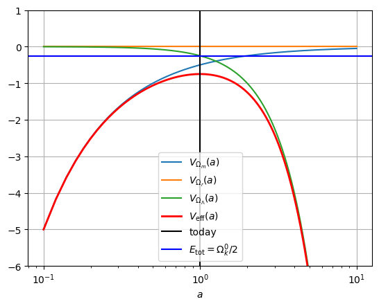
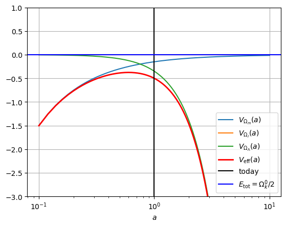
V e f f ( a ) = − 1 2 Ω m 0 a − 1 2 Ω Λ 0 a 2 V_{\rm eff}(a) = - \frac{1}{2}\frac{\Omega_m^0}{a} - \frac{1}{2}\Omega_\Lambda^0 a^2 V eff ( a ) = − 2 1 a Ω m 0 − 2 1 Ω Λ 0 a 2 In this universe model, we have Ω Λ 0 = Ω m 0 / 2 \Omega_\Lambda^0 = \Omega_m^0 / 2 Ω Λ 0 = Ω m 0 /2
V e f f ( a ) = − 1 2 Ω m 0 a − 1 4 Ω m 0 a 2 V_{\rm eff}(a) = - \frac{1}{2}\frac{\Omega_m^0}{a} - \frac{1}{4}\Omega_m^0 a^2 V eff ( a ) = − 2 1 a Ω m 0 − 4 1 Ω m 0 a 2 d V e f f d a = 0 ⇒ ( 1 a 2 − a ) Ω m 0 = 0 ⇒ a = 1 (today) \frac{\dd V_{\rm eff} }{\dd a}= 0 \Rightarrow \left(\frac{1}{a^2}-a\right)\Omega_m^0 = 0 \Rightarrow a=1\text{ (today)} d a d V eff = 0 ⇒ ( a 2 1 − a ) Ω m 0 = 0 ⇒ a = 1 (today) At a = 1 a=1 a = 1 t = 0 t=0 t = 0
1 = Ω m 0 + Ω Λ 0 + Ω k 0 ⇒ Ω k 0 = 1 − 3 2 Ω m 0 1 = \Omega_m^0 + \Omega_\Lambda^0 + \Omega_k^0 \Rightarrow \Omega_k^0 = 1 - \frac{3}{2}\Omega_m^0 1 = Ω m 0 + Ω Λ 0 + Ω k 0 ⇒ Ω k 0 = 1 − 2 3 Ω m 0 The model is spherical so Ω k 0 = − k c 2 / H 0 2 < 0 \Omega_k^0 = -k c^2 / H_0^2 < 0 Ω k 0 = − k c 2 / H 0 2 < 0 k = + 1 k=+1 k = + 1 Ω m 0 > 2 / 3 \Omega_m^0 > 2/3 Ω m 0 > 2/3 Ω m 0 = 1 \Omega_m^0=1 Ω m 0 = 1
Figure 1: Potential energies in the case of a spherical universe with Ω m 0 = 1 \Omega_m^0=1 Ω m 0 = 1
According to figure Figure 1 a = a 0 a=a_0 a = a 0
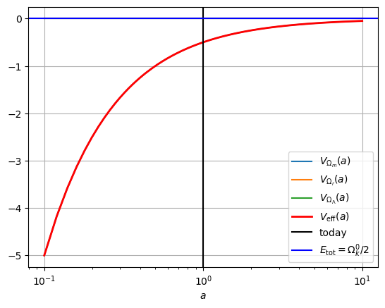
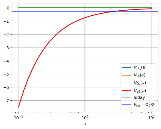
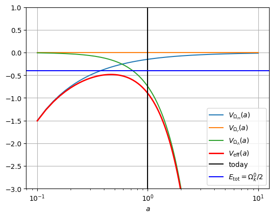
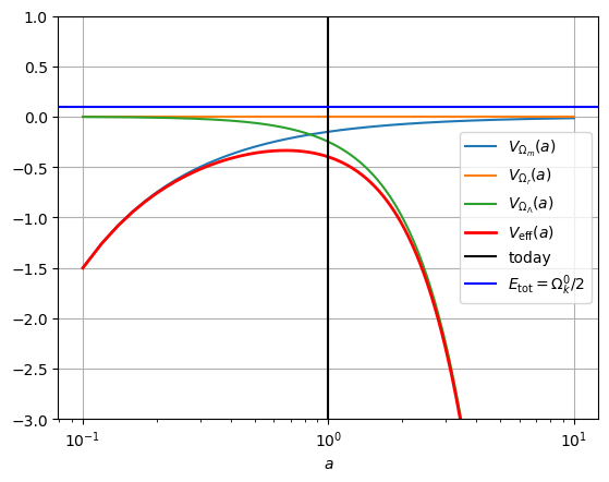
Table 1: Potential energies in the case of matter-only models with different curvatures: (top left), Ω m 0 = 1.5 ⇒ k = + 1 \Omega_m^0=1.5\Rightarrow k=+1 Ω m 0 = 1.5 ⇒ k = + 1 Ω m 0 = 0.5 ⇒ k = − 1 \Omega_m^0=0.5\Rightarrow k=-1 Ω m 0 = 0.5 ⇒ k = − 1
Ω m 0 = 1 ⇒ k = 0 \Omega_m^0=1\Rightarrow k=0 Ω m 0 = 1 ⇒ k = 0
Ω m 0 = 1.5 ⇒ k = + 1 \Omega_m^0=1.5\Rightarrow k=+1 Ω m 0 = 1.5 ⇒ k = + 1
Ω m 0 = 0.5 ⇒ k = − 1 \Omega_m^0=0.5\Rightarrow k=-1 Ω m 0 = 0.5 ⇒ k = − 1
In these models, the curvature is again given by:
1 = Ω m 0 + Ω k 0 ⇒ Ω k 0 = 1 − Ω m 0 ⇒ { k = + 1 if Ω m 0 > 1 k = 0 if Ω m 0 = 1 k = − 1 if Ω m 0 < 1 1 = \Omega_m^0 + \Omega_k^0 \Rightarrow \Omega_k^0 = 1 -\Omega_m^0 \Rightarrow
\left\lbrace\begin{array}{ll}
k=+1 & \text{ if } \Omega_m^0 > 1\\
k=0 & \text{ if } \Omega_m^0 = 1 \\
k=-1 & \text{ if } \Omega_m^0 < 1
\end{array}\right. 1 = Ω m 0 + Ω k 0 ⇒ Ω k 0 = 1 − Ω m 0 ⇒ ⎩ ⎨ ⎧ k = + 1 k = 0 k = − 1 if Ω m 0 > 1 if Ω m 0 = 1 if Ω m 0 < 1 By analyzing the three plots in figure Table 1 t → ∞ t\rightarrow \infty t → ∞
The transition scale factor is given by:
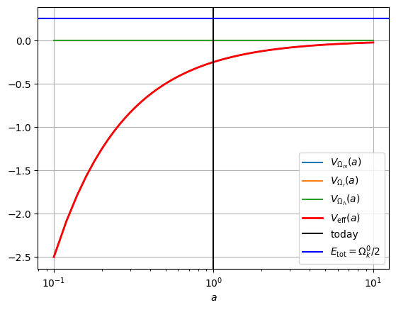
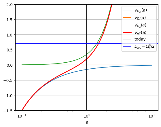
d V e f f d a = 0 → a ∗ = ( Ω m 0 2 Ω Λ 0 ) 1 / 3 \frac{d V_{\rm eff} }{da}= 0 \rightarrow a_* = \left(\frac{\Omega_m^0}{2 \Omega_\Lambda^0}\right)^{1/3} d a d V eff = 0 → a ∗ = ( 2 Ω Λ 0 Ω m 0 ) 1/3 Table 2: Potential energies in the case of Λ \Lambda Λ
Ω m 0 = 0.3 , Ω Λ 0 = 0.7 \Omega_m^0=0.3, \Omega_\Lambda^0=0.7 Ω m 0 = 0.3 , Ω Λ 0 = 0.7
Ω m 0 = 0.3 , Ω Λ 0 = 1.5 \Omega_m^0=0.3, \Omega_\Lambda^0=1.5 Ω m 0 = 0.3 , Ω Λ 0 = 1.5
Ω m 0 = 0.3 , Ω Λ 0 = 0.5 \Omega_m^0=0.3, \Omega_\Lambda^0=0.5 Ω m 0 = 0.3 , Ω Λ 0 = 0.5
Ω m 0 = 0.3 , Ω Λ 0 = − 0.7 \Omega_m^0=0.3, \Omega_\Lambda^0=-0.7 Ω m 0 = 0.3 , Ω Λ 0 = − 0.7
Depending on the parameter values, the transition scale occurs in the future or in the past. If the cosmological constant is positive, expanding universes have decelerated expansion and, after the transition scale, accelerated expansion. If the cosmological constant is negative, the universe must collapse after some time.
Why is the Universe therefore expanding today? This depends entirely on initial conditions, so in particular because the universe was born from a Big Bang. And why was there a Big Bang? One can let one’s imagination run free: brane collisions, God, pan-dimensional mice... but the answer is not (yet) given by physical sciences.
4 Evolution of cosmological parameters ¶ Figure 2: Evolution of cosmological parameters.
The integration of the first Friedmann equation by injecting the evolution properties of different fluids allows us to obtain the evolution of the scale factor as a function of time.
Whether with relativistic matter, non-relativistic matter or for an empty Universe, we obtain functions that increase with time since we measure H 0 > 0 H_0>0 H 0 > 0
Writing the first Friedmann equation in the form of an equation analogous to energy conservation in classical mechanics provides intuition about the evolution of a Universe as a function of the different components present. Among other things, non-relativistic matter restrains expansion through its attractive gravitational effect, while a positive cosmological constant leads to an acceleration of expansion in the future.
Planck Collaboration, Aghanim, N., Akrami, Y., Ashdown, M., Aumont, J., Baccigalupi, C., Ballardini, M., Banday, A. J., Barreiro, R. B., Bartolo, N., Basak, S., Battye, R., Benabed, K., Bernard, J.-P., Bersanelli, M., Bielewicz, P., Bock, J. J., Bond, J. R., Borrill, J., … Zonca, A. (2020). Planck 2018 results - VI. Cosmological parameters. A&A , 641 , A6. 10.1051/0004-6361/201833910 Balbinot, R., Bergamini, R., & Comastri, A. (1988). Solution of the Einstein-Strauss problem with a \ensuremathΛ term. \prd , 38 (8), 2415–2418. 10.1103/PhysRevD.38.2415 Martin, J. (2012). Everything You Always Wanted To Know About The Cosmological Constant Problem (But Were Afraid To Ask). Comptes Rendus Physique , 89. http://www.sciencedirect.com/science/article/pii/S1631070512000497%20http://arxiv.org/abs/1205.3365 Weinberg, S. (1989). The cosmological constant problem. Reviews of Modern Physics , 61 (1), 1–23. 10.1103/RevModPhys.61.1