There are two types of cosmological measurements: distance measurements, which map the expansion history of the Universe, and structure growth measurements, which describe the evolution of the Universe’s large-scale structures. The former are simple data that ultimately amount to measuring the evolution of the Hubble parameter . Two methods are used. The first method, which has been used historically, uses standard candles, via Type Ia supernovae. If we know that a category of astrophysical objects all have the same intrinsic luminosity, then if this object appears faint, it is located far away and we can deduce its distance from its apparent luminosity. The second method uses a standard ruler, i.e., an invariant characteristic length that can be measured throughout the history of the Universe. If this length appears smaller than it is today at a certain redshift , then knowing that it must not have evolved (or knowing how it evolved), we can find out its distance. This method is used in baryonic acoustic oscillations and the measurement of the angular power spectrum of the cosmic microwave background. The principle behind these two methods is illustrated in Figure 1.
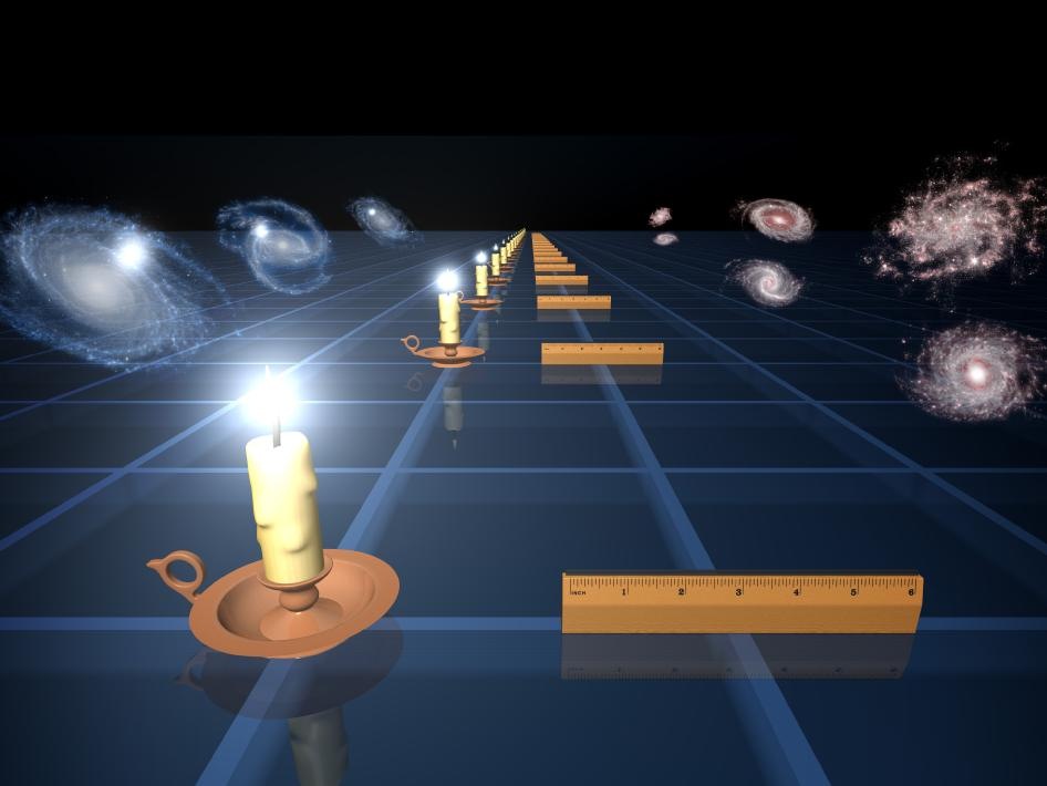
Figure 1:Principle of the measurement of the expansion of the Universe using standard candles (Type Ia supernovae) and a standard ruler (average distance between galaxies, derived from the average distance between overdensities of the cosmic microwave background).
1Principle of the standard candle method
The standard candle method is based on measuring the luminous fluxes from stars of identical intrinsic luminosity. To measure the speed of expansion of the Universe, we need luminosity distances associated with redshifts and thus construct a Hubble-Lemaître diagram.
The Apparent magnitude is a logarithmic scale that measures the luminosity of an object observed from Earth. It is based on the measurement of a luminous flux acquired with a telescope equipped with a photosensitive sensor (/s/m) or a bolometer (W/m), compared with a reference flux which sets the scale. Historically, the scale was based on a standard star, Vega in the constellation Lyra. To tie in with the 6 categories of magnitudes defined in ancient times, the apparent magnitude of a star is defined by:
The absolute magnitude is the flux we would receive from this source at a distance of :
In an ideal world, it would be enough to measure the fluxes of a collection of standard candles at redshifts and compare them to obtain a relationship between luminosity distance and redshift. The apparent magnitude of a standard candle at redshift is related to the expansion rate via the luminosity distance:
The quantity:
is the decrease in luminosity in magnitude linked to the distance of the star. If a standard candle is 2 times further away, then it appears 4 times less bright and its distance modulus increases by 1.5 magnitudes. By measuring the fluxes, we can thus estimate the relative distances between the standard candles.
The most important point to note in this formula is that the cosmological expansion speed is inscribed in the shape of the curve, and not in its normalization. The normalization of the curve depends notably on and . The standard candles method thus allows us to measure the evolution of the expansion of the Universe, without having to know their absolute luminosity ! On the other hand, if we know their absolute luminosity , then we can establish a scale of absolute distances and the normalization of the Hubble diagram gives access to the value of (Figure 2).

Figure 2:Distance modulus as a function of redshift for three cosmological models. A change in the parameters modifies the shape of the curve while the parameter modifies its normalization.
2Hubble diagram of supernovae
To establish a Hubble diagram at cosmological distances, we need sources of identical luminosities that are visible at very great distances. Galaxies are of varying sizes and therefore intrinsic luminosities too variable to play this role. However, Type Ia supernovae are stellar explosions whose luminosity is commensurate with that of a galaxy. They can therefore be visible from far away but only for a certain time.
Type Ia supernovae
Supernovae are classified into two types: gravitational and thermonuclear. The former are the best known: they correspond to the explosion of a massive star (more than 8 times the mass of the Sun) at the end of its life, leaving a dense and cold stellar core: a neutron star, or even a black hole in extreme cases. Type I supernovae are those that do not present hydrogen lines in their spectrum, while Type II supernovae contain them. Among Type I supernovae, those containing silicon are Type Ia, then the others Ib or Ic.
Stars with a mass less than end their lives as red giants. At the end of helium burning, the outer layers are dispersed into the interstellar medium as planetary nebulae (without necessarily producing an intense explosion), leaving the stellar core bare. The collapse of the core is stopped because of the degeneracy pressure of electrons (and not neutrons as for neutron stars) and its low mass (typically ). Its surface temperature remains very high for a long time (about ), hence its name of white dwarf. It is essentially composed of carbon and oxygen, the helium and hydrogen having been expelled into space. The typical radius of such an object is a few thousand kilometers (like a terrestrial planet).
This animation shows the explosion of a white dwarf, the extremely dense remnant of a star that can no longer burn nuclear fuel in its core. In this Type Ia supernova, the white dwarf’s gravity steals matter from a nearby stellar companion. When the white dwarf reaches a mass estimated at 1.4 times the current mass of the Sun, it can no longer support its own weight and explodes. Credit: NASA/JPL-Caltech
According to a study by the Very Large Telescope, about 75% of massive stars live in binary systems Sana et al., 2012. In some cases, a white dwarf can therefore be gravitationally bound to another star which, if it is sufficiently close, can see its outer layers sucked in by the gravity of the white dwarf. When the white dwarf has accumulated too much matter coming from its neighbor and approaches the Chandrasekhar mass (), it becomes unstable. The pressure and temperature conditions at the core of the white dwarf allow the reignition of carbon fusion. The white dwarf cannot expand and cool because of the degeneracy pressure of electrons, independent of temperature (quantum effect). The reaction runs away into a thermonuclear flame that vaporizes the star in a few seconds. The explosion enriches the interstellar medium with intermediate mass elements (oxygen, calcium, magnesium, silicon, sulfur) and elements from the iron family (nickel, cobalt). However, this explosion scenario remains only a hypothesis insofar as no proof yet exists. Other scenarios exist such as the merger of two white dwarfs Nomoto et al., 2013.
SNe Ia draw their energy from the disintegration of iron-group elements that were produced during the explosion Colgate & McKee (1969). The main radioactive element formed is :
since it is a simple stoichiometric combination of carbon and oxygen atoms, the most abundant atoms of a white dwarf. The nickel isotope then disintegrates into with a half-life of 6.1 days, which itself disintegrates into stable iron with a half-life of 77.3 days:
The total luminosity is estimated at , i.e., about that of a galaxy (see photographs Figure 4 and Figure 5). These are therefore objects a priori visible at cosmological distances. Since the explosion occurs systematically at the same stellar mass, roughly the same amount of material is ejected into space and emits the same amount of light. Moreover, since the composition of white dwarfs is very standard, the composition of the emitting matter is the same. They therefore all have roughly the same intrinsic total luminosity. However, they are also transient events: the duration of a supernova is a few tens of days. To capture one, you therefore need to look at the sky in the right place and at the right time.
Type Ia supernovae (SNe Ia) are the first cosmological probes that made it possible to measure the expansion of the Universe over cosmological distances, and discover its accelerated expansion Riess et al., 1998Perlmutter et al., 1999. The Nobel Prize in Physics was awarded in 2011 to Saul Perlmutter, Brian Schmidt and Adam Riess for this major discovery.
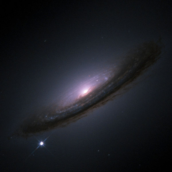
Figure 4:The supernova SN 1994D (the bright white dot in the bottom left of the image), in the spiral galaxy NGC4526.
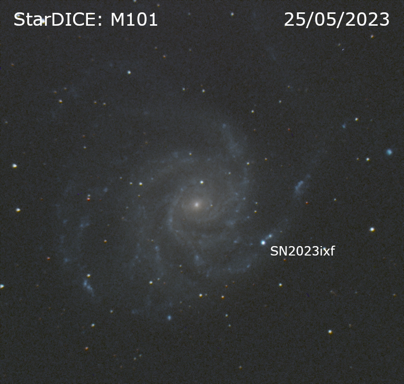
Figure 5:The supernova sn2023ixf discovered by the ZTF survey and photographed by the StarDICE telescope (Newton, diameter cm) in 4 filters on 25 May 2023.
Spectral sequences and light curves
A Type Ia supernova remains visible for about 40 days in the visible sky. To recognize its type, it must be observed in several colors and if possible acquire its spectrum. A sequence of spectra acquired on a Type Ia supernova is presented in Figure 7.
Series of images of a Type Ia supernova explosion. The supernova, SN 2015F, occurred in galaxy NGC 2442 in early March 2015, at a distance of about 80 million light-years from Earth. Daily images from February 2015 to October 2015 were combined to create this film. Images were taken with a 17-inch robotic telescope in Australia.
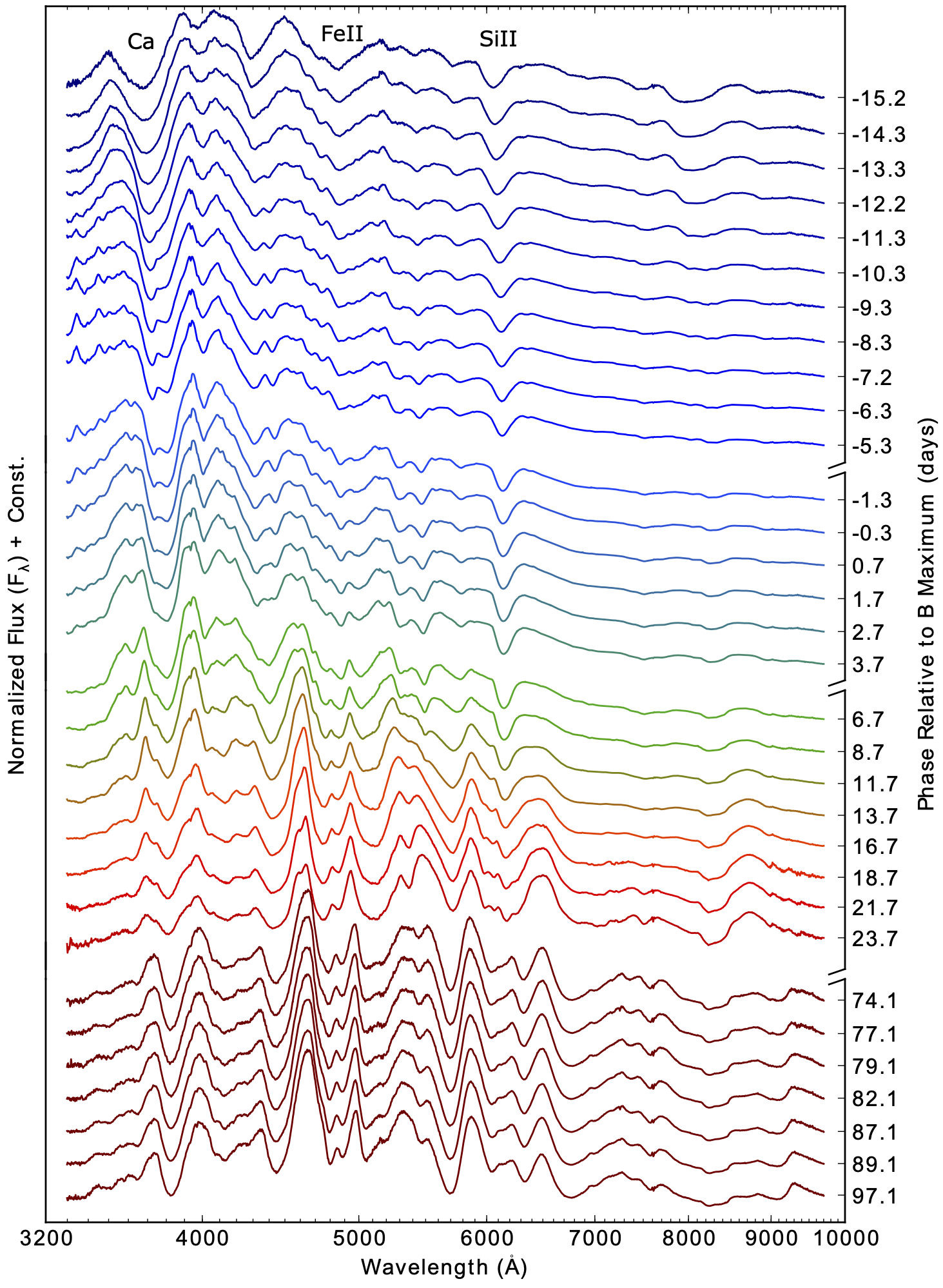
Figure 7:Spectro-temporal series of SN2011fe measured by the SNfactory survey Pereira et al., 2013. The names of the main components of the spectrum are indicated in the upper part of the figure.
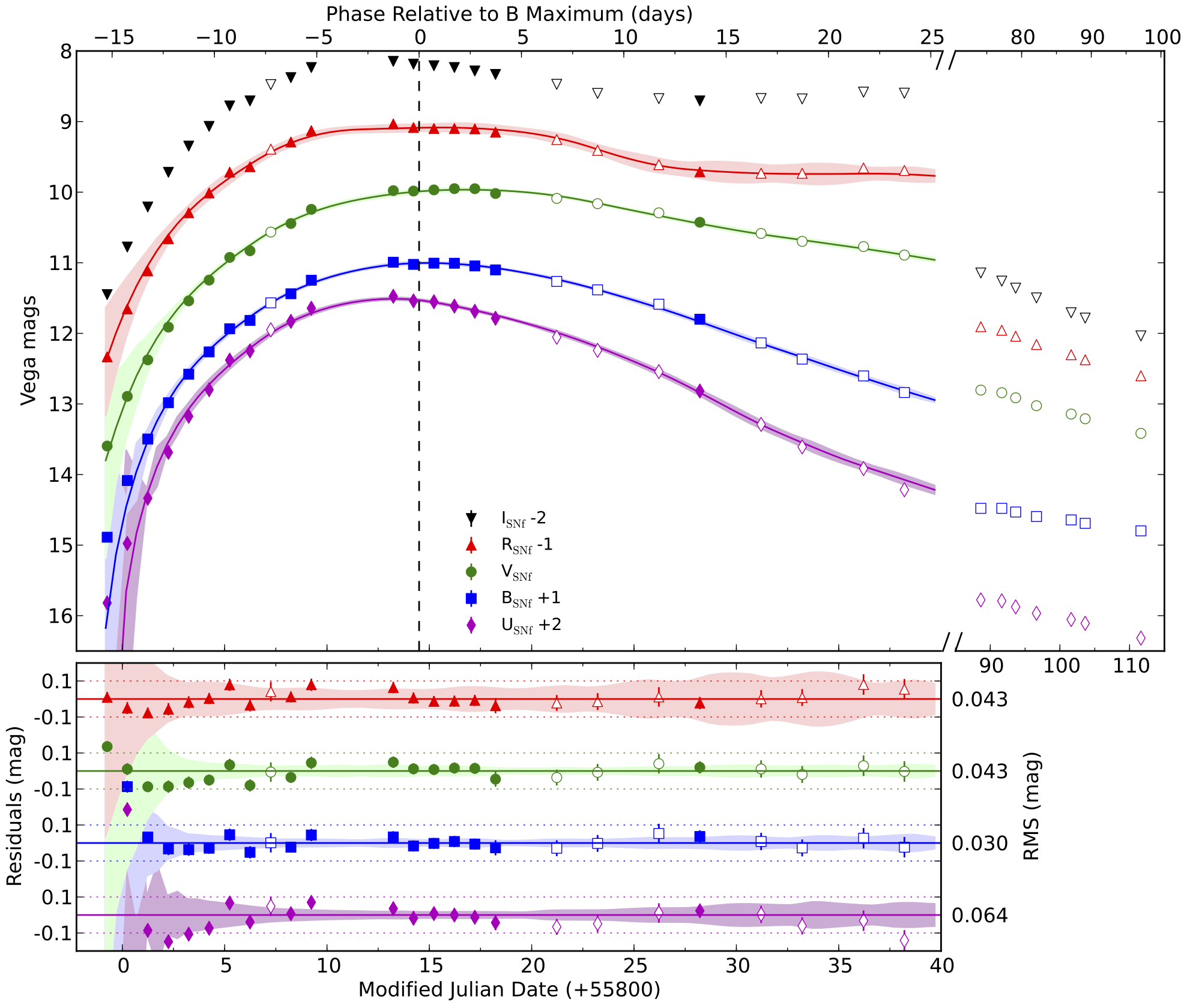
Figure 8:Light curves synthesized SN2011fe using the UBVRI filter set Pereira et al., 2013. Filled and open symbols correspond to photometric and non-photometric nights respectively. The results of a simultaneous SALT2 fit of UBVR in the range in the phase interval days are represented by solid lines, with the corresponding residuals (SALT2 - SNf) on the lower panel. The shaded areas represent the error of the SALT2 model. The break in the time axis corresponds to the gap of days in the follow-up during which SN2011fe was not visible during the night from Hawaii. Note the change in scale of the extended time axis covering the late observations.
In practice, we do not have spectral sequences as precise as the one presented in Figure 7 for each detected supernova, because this costs too much observation time on the world’s largest telescopes equipped with spectrographs. Only the SNFactory survey has dedicated a spectrograph to the systematic spectral study of supernovae. As a general rule, if possible, only one spectrum of the supernova is acquired around its maximum luminosity (because it is easier) in order to verify that it is indeed a Type Ia (identification spectrum), with a spectrograph that does not need to have high resolution to identify the main lines of the thermonuclear explosion. Later, a spectrum of the host galaxy is taken to measure its redshift precisely if it is not already known, with a higher resolution spectrograph (redshift spectrum).
The main information available on a Type Ia supernova is therefore its light curve, i.e., the temporal sequence of luminous fluxes, measured by a telescope with different band-pass filters equipping the telescope’s camera Figure 8.
It is therefore necessary to define an instant at which to compare the brightness of standard candles and a reference filter. For practical reasons, we use the magnitudes at maximum emission as a reference. For historical reasons, we use the Johnson B band as a reference filter. The magnitude of the maximum luminosity of a Type Ia supernova observed in the B band is therefore used as a standard candle, or at least as standardizable.
Photometric systems
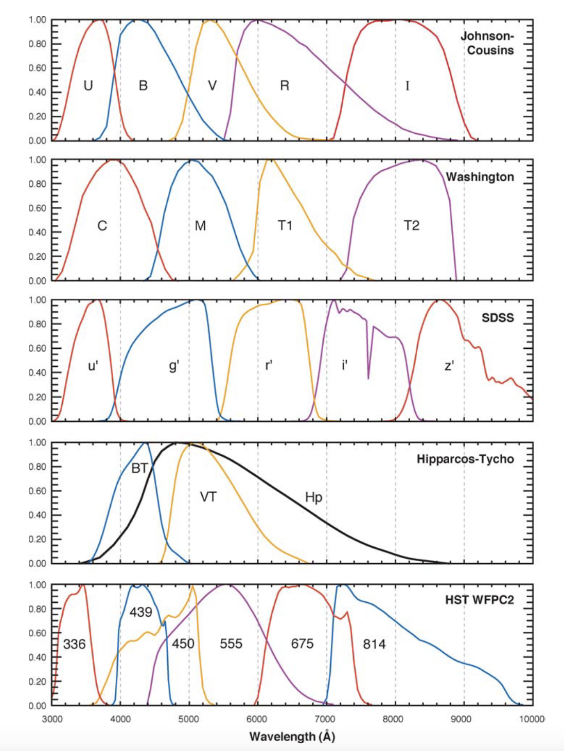
Figure 9:Band-pass filters for different photometric systems Bessell, 2005.
Astrophysical and cosmological surveys in photometry are interested in measuring the color of objects to access their physical properties. For this, telescopes are equipped with band-pass filters, whose shapes and positions depend on the technologies used and the needs of the survey.
A standard photometric system is defined by a list of standard magnitudes and colors measured at specific bandwidths for a set of stars well distributed across the sky. The observed magnitudes are corrected to account for the attenuation of Earth’s atmosphere away from the zenith, and the data are then normally extrapolated to zero air mass (outside the atmosphere).
The UBV system is one of the oldest and most widely used standard photoelectric photometric systems Johnson & Morgan (1953). The B band was designed to approximate the raw photographic magnitude (minus UV), while the V band was designed to approximate the visual magnitude system. The photometric systems of modern SDSS and LSST surveys instead use interference filters named ugrizy in the visible and near infrared.
Rest frame magnitude
The luminous fluxes expressed in (/s/m) or (W/m) are called bolometric[1] because they are integrated over the entire spectrum. Unfortunately, the ability to measure this quantity depends on the sensor used. In the visible and infrared, sensors are based on the photoelectric effect so they are transparent above a certain wavelength. In the visible and infrared, measured fluxes cannot be bolometric.
Moreover, much information can be derived from measuring the color of an object, such as the type of supernova: for this it must be observed through different band-pass filters and to compare the fluxes.
We introduce the spectral energy density of a star expressed[2] in W/m/nm. Let us note the transmission of the instrument equipped with a filter . The measured flux is then:
where is the wavelength of incident photons. Then the definition of apparent magnitude for a filter becomes:
with the spectral flux density of the reference source (Vega for example). The absolute magnitude in filter is the magnitude of the star in filter if observed in its rest frame at :
with the spectral luminosity (in W/nm).
We note the transmission of filter B in the Johnson UBV photometric system (see box). Then we define:
The absolute magnitude in band is:
However, not all telescopes are equipped with a B filter. Moreover, and this is the main reason, the emission maximum shifts in wavelength with the redshift so it would be necessary to redshift the B filter to capture the same portion of spectrum (Figure 10). Since we want to compare only the effect of distance to map , these wavelength shift effects must nevertheless be removed to standardize and compare the observed flux at maximum emission. Historically, for Type Ia supernovae, cosmologists establish apparent magnitudes in B band in the supernova’s rest frame. The magnitude is therefore the apparent magnitude in the rest frame in B band, as if there were no expansion but only a distance effect.
The standard candle is the maximum emission of Type Ia supernovae in the band as if observed in their rest frame.
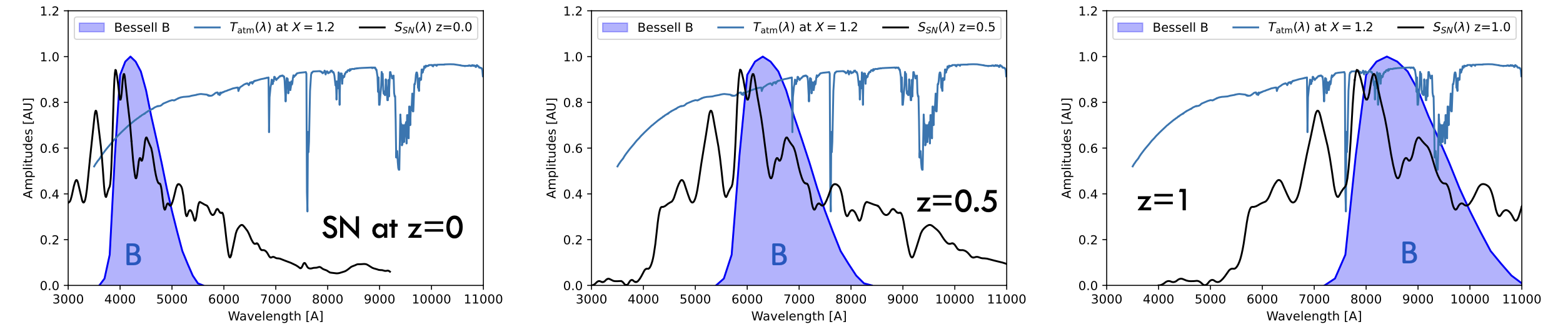
Figure 10:Apparent magnitudes in band for supernovae at different redshifts: they correspond to the integral of the supernova’s spectral density at its maximum in the redshifted band.
Since it is not possible to make an observation in the supernova’s rest frame, this magnitude must be calculated from observations in arbitrary filters and a spectrophotometric model of the supernova.
Spectrophotometric model
The spectrophotometric model will be the data of the spectral density as a function of time , determined on the data (the collection of light curves and spectra available). Suppose we are able to obtain it, after training on the data, as with the SALT2 model Guy et al., 2007. How can we transform the observed apparent magnitudes into B band magnitudes in the rest frame ?
First, we must study the effect of redshift on spectral densities. The flux and the intrinsic luminosity (in W) of a star located at redshift are related by:
with the luminosity distance. All photons received in a narrow logarithmic frequency range centered on the observed wavelength have been emitted in an equally narrow wavelength range also centered on . Equation (12) thus relates the spectral flux densities to the spectral luminosities in the presence of a redshift Condon & Matthews, 2018:
This relation gives the link between the spectral flux density observed at and the spectral luminosity density emitted at .
Now, let us search how to transform the observed magnitudes into magnitudes , from the definition of apparent magnitude in band :
Let us define the -correction in bands and Hogg et al., 2002:
Then the apparent magnitude can be decomposed into three terms:
and the magnitude is calculated from the observations and the calculated -correction:
The -correction represents the magnitude correction that must be applied if we observed the star in its rest frame and with another filter. After applying the -correction, the Hubble diagram is simply modeled by:
an equation very similar to (3). The left member represents the magnitudes acquired by the telescope and transformed into B band at rest and at maximum. The right member represents the explanatory cosmological model. For SNe Ia, Betoule et al., 2014. We can see that the distance dependence is entirely contained in the distance modulus , but notice that there is an additional redshift dependence in the -correction. It is therefore necessary to know how to correctly model so as not to introduce redshift bias in the Hubble diagram.
Unfortunately, the -correction depends on a certain number of ingredients that must therefore be known beforehand to calculate it:
the redshift , to be inferred from a spectrum;
the spectral density of the supernova, to be constructed by a spectrophotometric model fitted to the measured spectral sequences (as in Figure 7) like SALT2 Guy et al., 2007;
the reference spectral density , to be established by measurement (Hayes et al. (1975), Souverin et al. (2024)) or stellar atmosphere modeling Bohlin et al. (2014);
the transmission of the telescope filters , or even the atmospheric transmission of the site .
To obtain a measurement of the dark energy equation of state parameter at the percent level, each of these ingredients must therefore be established to better than the percent. Today, the dominant uncertainties on the measurement of by Type Ia supernovae are the systematic uncertainties of photometric calibration, i.e., knowledge of the bandwidth of instrument filters as well as knowledge of reference fluxes Betoule et al., 2013Scolnic et al., 2018.
Standardization
After -correction, we can compare the magnitudes to a cosmological model. With the JLA data from the SuperNova Legacy Survey, we obtain the Hubble diagram Figure 11.
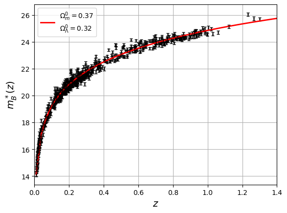
Figure 11:Hubble diagram of the 740 SNeIa from the SNLS survey, compared to a CDM model with and .
Around the diagram, we observe that the residuals to the Hubble diagram have a dispersion of mag, greater than the measurement errors. If we plot these residuals as a function of the color or the normalized duration of the supernova, we see that they are correlated (Table 1).
Table 1:Residuals to the Hubble diagram colored as a function of the normalized duration (left) or the color (right).
Source:Type Ia supernovae 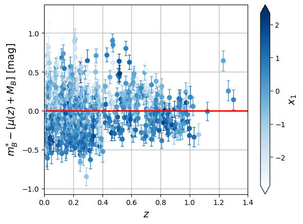 | Source:Type Ia supernovae 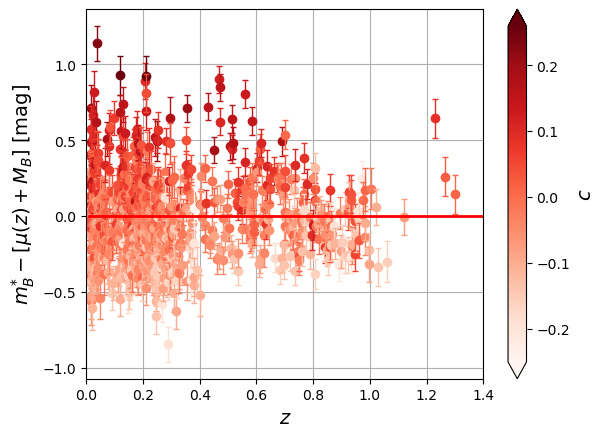 |
There is therefore a variability of supernovae that has not been taken into account in our spectrophotometric model so far.
We observe that the longer the light curve lasts in time, the brighter it is at its maximum (brighter-slower rule). Moreover, the bluer the SNIa are, the brighter they are as well (brighter-bluer rule). There is also an environmental effect that links the brightness of the supernova and the mass of the host galaxy.

Figure 12:Light curves of SNe Ia from the JLA dataset of the SNLS survey colored as a function of or Nicolas, 2022.
The light flux is linked to the production and decay of nickel Ni. The two relations presented above can thus be explained qualitatively: the more Ni the SNIa produces, the brighter it will be and the more it will contain FeII and CoII ions emitting in the blue, but also the more it will be opaque (so the emission of photons by scattering will be delayed, so the SNIa will shine longer) Kasen & Woosley, 2007.
SNe Ia are therefore not so standard, because their light curves depend on the amount of Ni available at the origin. Nevertheless, without correcting this intrinsic dispersion, the teams of the Supernova Cosmology Project (SCP) led by Saul Perlmutter and the High-z Supernova Search Team led by Brian Schmidt were able to demonstrate the existence of an accelerated expansion Riess et al., 1998Perlmutter et al., 1999. This dispersion is problematic for improving measurements of the expansion of the Universe at the percent level. Nevertheless, it can be described empirically by two linear relations for and with coefficients and respectively. For the host mass, we adjust a parameter increasing the magnitude for supernovae located in galaxies of mass greater than .
These three empirical relations add three additional parameters , and to also fit on the data Tripp & Branch (1999):
After this standardization, the dispersion in the Hubble diagram is reduced to mag which increases the precision on cosmological parameters.
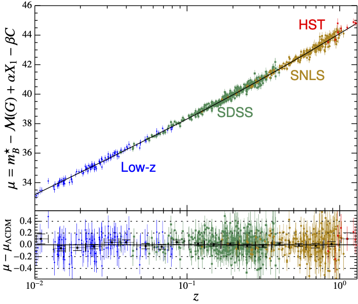
Figure 13:Hubble diagram of supernovae from the JLA catalog. The black curve represents a CDM model fitted to the data. A model without dark energy would appear significantly below the curve described by the data (mag at ).
Calibrations
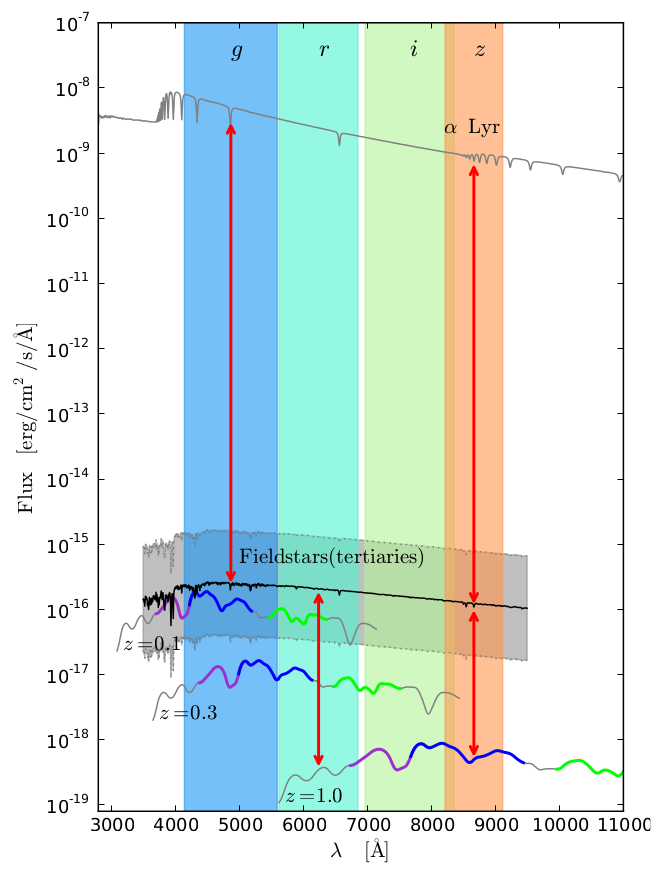
Figure 14:Strategies for calibrating the measurement of the luminous flux of tertiary stars (secondary stars are not represented). The redshifted band is represented by a thick blue line on the spectra of SNe Ia.
State of the art
3Local measurement of 
TODO: See, read and study https://
The distance modulus allows us to measure the relative distance between SNe Ia, which provides crucial information on dark energy. However, the absolute distance of SNe Ia cannot be obtained by this method: there is a degeneracy between the luminosity of SNe Ia and during estimation. To break this degeneracy, the cosmic distance ladder is used. This method involves a series of overlapping distance measurements using various astronomical objects and techniques, as illustrated in figure 12 of Riess et al. (2022). By anchoring the distances of SNe Ia to distances measured independently by the cosmic distance ladder, we can disentangle the absolute magnitude of SNe Ia from that of H0. In what follows, we will discuss the different steps of this distance ladder.
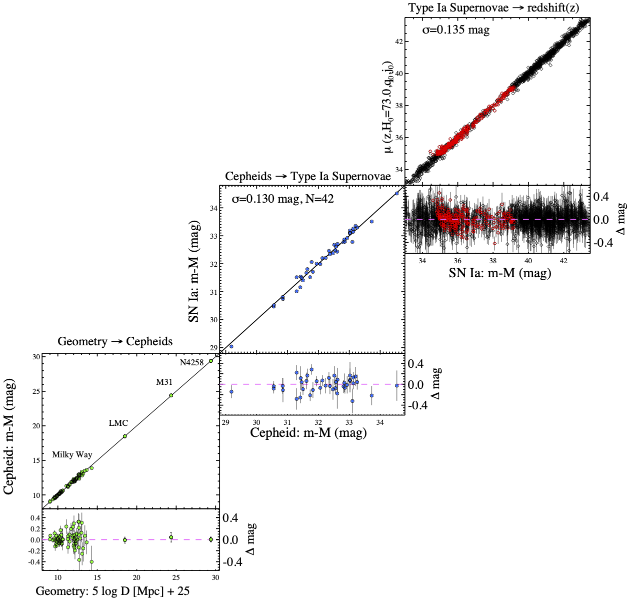
Figure 15:Astrophysical distance ladder Riess et al., 2022. Measurements of orbital parameters in the Solar System allow calibrating the measurement of stellar distances by the parallax method. The distance of certain Cepheid stars is measured by parallax which allows establishing a relation between the flux of cepheids, their period of luminosity and their distance (lower square). The distance obtained by the luminosity of Cepheids in nearby galaxies allows calibrating the intrinsic luminosity of SNe Ia exploding in a galaxy containing Cepheids (intermediate square). Once the intrinsic luminosity of SNe Ia is known, measuring the slope of the distance-redshift relation for distant supernovae (but not too distant) allows access to .
Parallax measurement
When a foreground star is observed from two opposite positions, A and B, on Earth’s orbit around the Sun, it appears to move relative to the background star field toward positions A’ and B’. This apparent shift is called parallax. The distance between Earth and the Sun is defined as an astronomical unit (AU), i.e., the average between the two semi-axes of Earth’s elliptical orbit. With this distance, and by measuring the apparent displacement of the star’s position, we can calculate by trigonometry the distance between the observer and the star. This phenomenon is known as parallax. Parallax measurements made by Gaia reach a precision of 0.04 mas Luri et al. (2018). This method constitutes the first rung of the cosmic distance ladder.
Cepheids
Cepheids are a type of star that pulsates radially, undergoing regular variations in diameter and temperature. These pulsations result in luminosity changes with a well-defined and stable period and amplitude. They were discovered by Henrietta Swan Leavitt Leavitt, 1907, who highlighted the correlation between the star’s diameter and temperature.
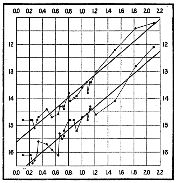
Figure 16:Relation between the magnitude of the minima (lower curve) and maxima (upper curve) of Cepheid light curves as a function of the logarithm of their pulsation period, according to Leavitt & Pickering (1912).
The magnitude of the maxima or minima of a Cepheid’s light curve is proportional to the logarithm of its pulsation period. This law is known as Leavitt’s law, and figure 2 of Leavitt & Pickering (1912), illustrates this relation (Figure 16).
By observing Cepheids close enough to use the parallax method for distance estimation, we can calibrate the absolute magnitude of Cepheids, and therefore their intrinsic period-luminosity relation. Due to the stability of their period-luminosity function, this calibration can then be applied to all Cepheids, allowing us to measure their luminosity distance in other galaxies where the parallax method is not feasible. Therefore, Cepheids serve as the first standard candle in the cosmic distance ladder, allowing us to determine the distance of other galaxies, as shown in the central graph of Figure 15.
Type Ia supernovae
Once the period-luminosity function of Cepheids is calibrated, this calibration is transferred to SNe Ia. To estimate the distance of a galaxy using a Cepheid, it must be resolved relative to other luminous sources in the galaxy and its photometry must be performed (Figure 17). By measuring its pulsation period, we deduce its intrinsic luminosity and therefore the distance of the host galaxy.
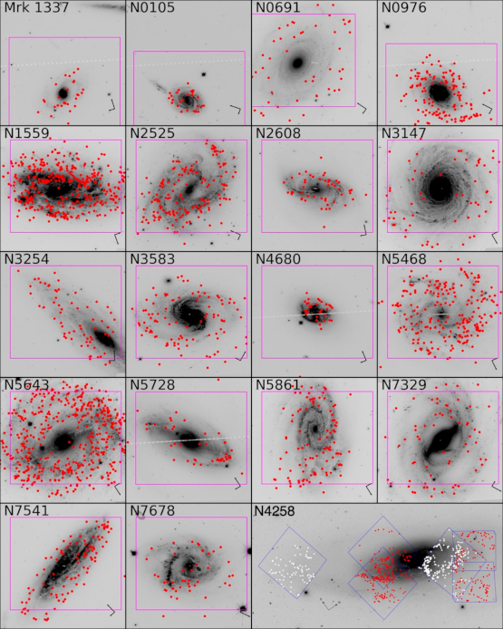
Figure 17:Identification of Cepheids (red dots) in 18 galaxies where SNe Ia were observed as well as in the maser NGC4258, by the SHOES survey of the Hubble Space Telescope (from Riess et al. (2022)).
Next, observing an SN Ia in the same galaxy allows knowing its intrinsic luminosity since the distance is known via the Cepheid. Riess et al. (2022) reports the observation of 42 SNe Ia in 37 calibrated hosts. These SNe Ia are represented in the central square of Figure 15, allowing calibration of the absolute magnitude of SNe Ia. Finally, the upper square plots a Hubble diagram of SNe Ia, which is directly linked to the geometric distance estimation by the parallax method.
With this sample, Riess et al. (2022) reports a measurement of of km/s/Mpc, in tension at more than with the extrapolation of measurements from Planck Collaboration et al. (2020). There is therefore a disagreement between measurements made on the CMB (young universe, distant) and measurements made with SNe Ia (recent universe, local). Multiple sources of systematic errors have been investigated but so far none of them seem to resolve the tension. Alternative independent measurement methods are also being implemented to decide between SNe Ia proponents and CMB proponents, such as for example the use of neutron star mergers observed in optical and gravitational waves. Also, new physics models are in competition to reconcile the young universe and the recent universe (-Olympics: Schöneberg et al. (2022)).
A bolometric sensor is capable of absorbing photons and measuring their energy regardless of their wavelength (for example by measuring the heating of a material). In contrast, a photonic sensor based on the photoelectric effect becomes transparent at long wavelengths, when the photon energy falls below the electron emission threshold.
Or in frequency expressed in W/m/Hz.
- Sana, H., de Mink, S. E., de Koter, A., Langer, N., Evans, C. J., Gieles, M., Gosset, E., Izzard, R. G., Le Bouquin, J.-B., & Schneider, F. R. N. (2012). Binary interaction dominates the evolution of massive stars. Science (New York, N.Y.), 337(6093), 444–446. 10.1126/science.1223344
- Nomoto, K., Kamiya, Y., & Nakasato, N. (2013). Type Ia Supernova Models and Progenitor Scenarios. Proceedings of the International Astronomical Union, 7(S281), 253–260. 10.1017/S1743921312015165
- Colgate, S. A., & McKee, C. (1969). Early Supernova Luminosity. The Astrophysical Journal, 157, 623. 10.1086/150102
- Riess, A. G., Filippenko, A. V., Challis, P., Clocchiatti, A., Diercks, A., Garnavich, P. M., Gilliland, R. L., Hogan, C. J., Jha, S., Kirshner, R. P., Leibundgut, B., Phillips, M. M., Reiss, D., Schmidt, B. P., Schommer, R. A., Smith, R. C., Spyromilio, J., Stubbs, C., Suntzeff, N. B., & Tonry, J. (1998). Observational Evidence from Supernovae for an Accelerating Universe and a Cosmological Constant. The Astronomical Journal, 116(3), 1009–1038. 10.1086/300499
- Perlmutter, S., Aldering, G., Goldhaber, G., Knop, R. A., Nugent, P., Castro, P. G., Deustua, S., Fabbro, S., Goobar, A., Groom, D. E., Hook, I. M., Kim, A. G., Kim, M. Y., Lee, J. C., Nunes, N. J., Pain, R., Pennypacker, C. R., Quimby, R., Lidman, C., … Project, T. S. C. (1999). Measurements of Ω and Λ from 42 High-Redshift Supernovae. The Astrophysical Journal, 517(2), 565–586. 10.1086/307221
- Pereira, R., Thomas, R. C., Aldering, G., Antilogus, P., Baltay, C., Benitez-Herrera, S., Bongard, S., Buton, C., Canto, A., Cellier-Holzem, F., Chen, J., Childress, M., Chotard, N., Copin, Y., Fakhouri, H. K., Fink, M., Fouchez, D., Gangler, E., Guy, J., … Wu, C. (2013). Spectrophotometric time series of SN 2011fe from the Nearby Supernova Factory. Astronomy & Astrophysics, 554, A27. 10.1051/0004-6361/201221008
- Bessell, M. S. (2005). Standard Photometric Systems [Journal Article]. Annual Review of Astronomy and Astrophysics, 43(Volume 43, 2005), 293–336. https://doi.org/10.1146/annurev.astro.41.082801.100251
- Johnson, H. L., & Morgan, W. W. (1953). Fundamental stellar photometry for standards of spectral type on the revised system of the Yerkes spectral atlas. The Astrophysical Journal, 117, 313. 10.1086/145697
- Guy, J., Astier, P., Baumont, S., Hardin, D., Pain, R., Regnault, N., Basa, S., Carlberg, R. G., Conley, A., Fabbro, S., Fouchez, D., Hook, I. M., Howell, D. A., Perrett, K., Pritchet, C. J., Rich, J., Sullivan, M., Antilogus, P., Aubourg, E., … Ruhlmann-Kleider, V. (2007). SALT2: using distant supernovae to improve the use of type Ia supernovae as distance indicators. Astronomy and Astrophysics, 466(1), 11–21. 10.1051/0004-6361:20066930
- Condon, J. J., & Matthews, A. M. (2018). ΛCDM Cosmology for Astronomers. Publications of the Astronomical Society of the Pacific, 130(989), 073001. 10.1088/1538-3873/aac1b2
- Hogg, D. W., Baldry, I. K., Blanton, M. R., & Eisenstein, D. J. (2002). The K correction.
- Betoule, M., Kessler, R., Guy, J., Mosher, J., Hardin, D., Biswas, R., Astier, P., El-Hage, P., Konig, M., Kuhlmann, S., Marriner, J., Pain, R., Regnault, N., Balland, C., Bassett, B. A., Brown, P. J., Campbell, H., Carlberg, R. G., Cellier-Holzem, F., … Wheeler, C. J. (2014). Improved cosmological constraints from a joint analysis of the SDSS-II and SNLS supernova samples. 30. http://arxiv.org/abs/1401.4064
- Hayes, D. S., Latham, D. W., & Hayes, S. H. (1975). Measurements of the monochromatic flux from VEGA in the near-infrared. The Astrophysical Journal, 197, 587. 10.1086/153547
- Souverin, T., Neveu, J., Betoule, M., Bongard, S., Blanc, P. E., Tanugi, J. C., Dagoret-Campagne, S., Feinstein, F., Ferrari, M., Hazenberg, F., Juramy, C., Guillou, L. L., Van Suu, A. L., Moniez, M., Nuss, E., Plez, B., Regnault, N., Sepulveda, E., & Sommer, K. (2024). How the StarDICE photometric calibration of standard stars can improve cosmological constraints? arXiv. 10.48550/ARXIV.2411.03256
- Bohlin, R. C., Gordon, K. D., & Tremblay, P.-E. (2014). Techniques and Review of Absolute Flux Calibration from the Ultraviolet to the Mid-Infrared. Publications of the Astronomical Society of the Pacific, 000–000. 10.1086/677655