1Electromagnetic emissions on cosmic scales
Energy density, surface brightness, flux density and luminosity
An observable directly related to the energy density of an isotropic field of relativistic particles is the sky surface brightness. Following the notation of Rybicki & Lightman (1986), the bolometric surface brightness or bolometric intensity, , is defined as the energy passing through a surface during a time and coming from a solid angle :
with .
The energy density of the field of relativistic particles, , in a volume is such as , so that the average intensity integrated over the sphere is
Following again Rybicki & Lightman (1986), the energy density of a field of particles with momentum between and depends on the number of particles per phase volume, as
is invariant under a Lorentz transformation. Indeed is countable and thus invariant. Under a boost along the x-axis from the observer’s frame (K) to the comoving frame (K’) towards, one finds (length contraction) and for particles with fixed energy (total momentum fixed between and ). Thus is invariant, quod erat demonstrandum.
One finds
so that
The multi-wavelength spectrum of the universe
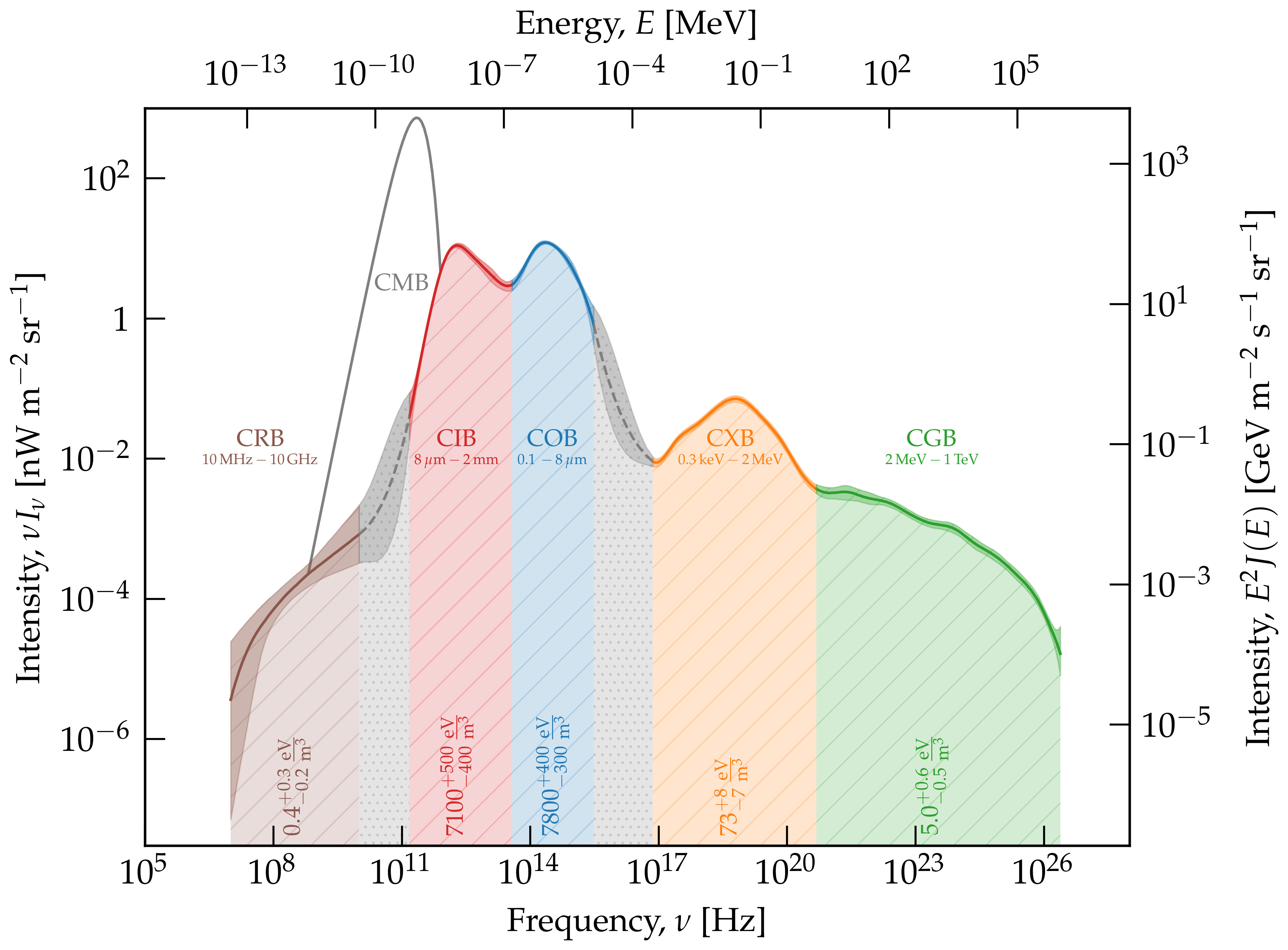
Figure 1:The multi-wavelength extragalactic spectrum. Adapted from this page.
The broadband emission from all galaxy populations (and from sources within these galaxies) is responsible for the spectrum of the universe shown in Figure 1. In particular, electromagnetic radiations include the cosmic radio background (CRB) from both active and star-forming galaxies, the cosmic infrared and optical backgrounds (CIB and COB) mostly from nucleosynthesis and dust emission in star-forming galaxies, the cosmic X-ray background (CXB) from active galaxies and the cosmic gamma-ray background (CGB) from jetted active galaxies. The differential measurements of these cosmic backgrounds are of fundamental value: they reflect our knowledge of the distribution of light emitted by star formation, accretion and ejection integrated since the formation of the first astrophysical sources. Although these emissions are only a negligible part of the cosmic energy inventory, they provide us with a cosmological consistency test that is essential for understanding the content and evolution of the post-recombination universe Fukugita & Peebles, 2004.
The values indicated by vertical text in Figure 1 correspond to the energy density of each component, i.e. the integral of the specific intensity multiplied by . In particular, it can be verified that the expected energy density from the nucleosynthesis and accretion processes calculated in the previous chapter, i.e. , is found nearly in its entirety in the COB and CIB. The energy density from ejection processes around supermassive black holes, expected at , is found in the CGB.
The measurements shown in Figure 1 also quantify the degree of darkness of the night sky once the foregrounds are subtracted. It is the history of their emission that provides the solution to the Olbers paradox. The present intensity of these backgrounds determines the darkness (or rather grayness) of the night sky, once all foregrounds (Solar System, Milky Way) have been removed. We can understand the extragalactic backgrounds at all electromagnetic wavelengths, the so-called extragalactic background light, using synthetic models of galaxy populations. Some unknowns in the extragalactic background light, including tensions between measurements, are nonetheless still the subject of active research Biteau, 2025.
Light emission is fundamentally the result of heating, acceleration and decay of matter. We will explore in the next section the knowledge established with photons, in particular through multi-wavelength observations of gamma-ray sources. We will also explore in the following lessons to which extent this multi-wavelength knowledge allows us to understand extragalactic backgrounds observed today with other messengers, in particular the extragalactic neutrino background (ENB) between TeV and PeV and the extragalactic cosmic-ray background (ECRB) between PeV and EeV.
2Electromagnetic emission of non-thermal sources
Multi-wavelength astronomy
The development of radio astronomy around the Second World War led to the emergence of multi-wavelength astronomy as a powerful tool for understanding the Milky Way and extragalactic sources. Karl Jansky first used this approach for Galactic observations in the 1930s, and from the 1960s onwards, Martin Schmidt and others employed it to study the first active galactic nuclei, known as quasars at the time. The subsequent emergence of X-ray and gamma-ray astronomy in the 1970s and 1990s, respectively, has led to our current understanding of non-thermal emitters — astrophysical sources that emit radiation beyond the optical and infrared spectrum.
Figure 2 provides a multi-wavelength view of the entire sky in Galactic coordinates. In this spherical coordinate system, the Galactic centre is in the middle of the map and the Galactic plane separates the northern and southern Galactic hemispheres. Note that the skymaps are shown as a function of decreasing Galactic longitude, ranging from on the left to on the right. This is the opposite of how we represent the Earth (i.e. with increasing longitude from left to right), because we are observing the sphere from within when we look at the sky.
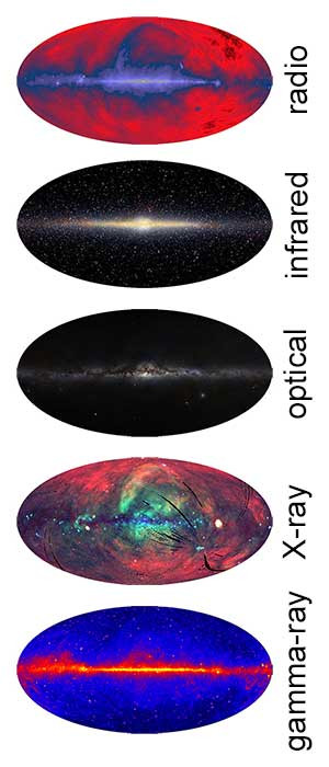
Figure 2:Multiwavelength view of the sky in Galactic coordinates. From this page.
Much of the radio emission shown in Figure 2 originates from high-energy electrons and positrons radiating within the magnetic field of the Milky Way. Shock waves in supernova remnants also produce intense radio emissions near these sources. Most of the infrared emission comes from relatively cool stars located in the disc and bulge of the Milky Way. Interstellar dust is relatively transparent at these wavelengths. At visible wavelengths (between 0.4 and 0.6 microns), strong absorption by gas and dust clouds limits the depth of observations. As a consequence, the visible light along the Galactic plane mainly originates from stars located a few kiloparsecs from the Sun. The composite X-ray image is reconstructed from bands centred at 0.25, 0.75 and 1.5 keV (red, green and blue, respectively). The hot, shocked gas in the Milky Way emits low-energy X-rays (also known as ‘soft X-rays’). The interstellar medium strongly absorbs soft X-rays, enabling us to perceive cold clouds of interstellar gas as shadows against the X-ray emission background. The black areas indicate gaps in the survey.
The gamma-ray image includes all photons with energies above 1 GeV. At these high energies, much of the gamma-ray emission along the Galactic plane originates from interactions of cosmic rays with hydrogen and helium nuclei in the interstellar medium. Bright, point-like sources are observed along the Galactic plane, such as the Vela, Geminga and Crab pulsars, which are located at longitudes of about , and , respectively. Point-like sources are also found outside the Galactic plane, primarily in the form of jetted active galactic nuclei. A more detailed introduction to the observations in each band, from which the previous two paragraphs are adapted, can be found on this page.
Zooming in on a square measuring approximately 0.1° centred on Galactic coordinates of l = -175.44° and b = -5.78° reveals in Figure 3 the emission surrounding the Crab pulsar. This extended emission is known as the Crab Nebula. The Crab Nebula is the result of a core-collapse supernova that exploded in 1054 AD. The pulsar at the heart of the nebula has a period of about 33 milliseconds. The rotation of the neutron star powers the radiation observed in the pulsar wind nebula.
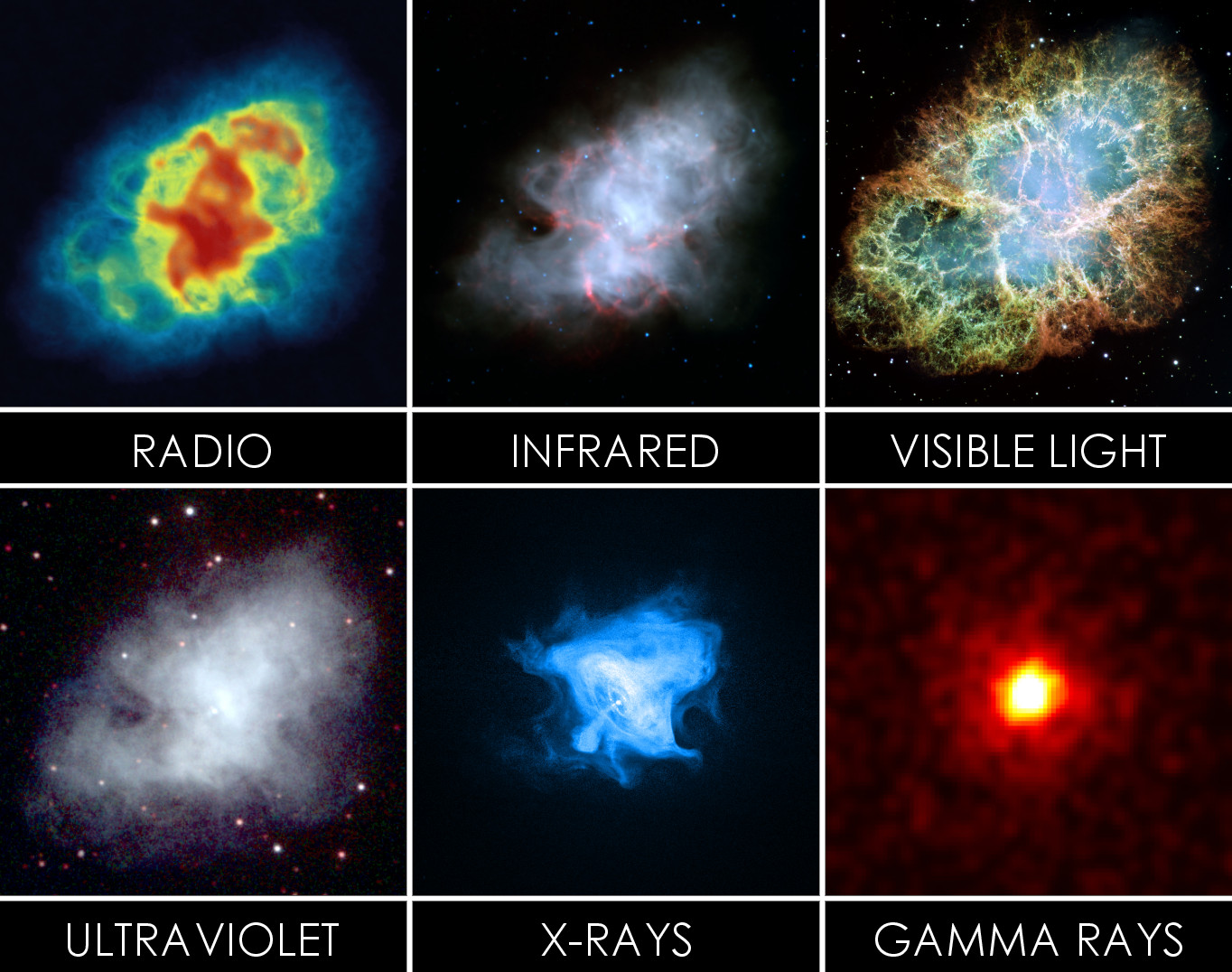
Figure 3:Multiwavelength view of the Crab Nebula. From this page.
In Figure 3, radio observations depict the pulsar wind nebula in red and the emission of free electrons in green. The blue-white region in the infrared image corresponds to electrons trapped in the magnetic field, while the red filaments reveal the rest of the star’s original outer layers. The network of filaments is clearly visible in the optical image, surrounding the bluish core of the pulsar wind nebula. The Crab Nebula extends slightly further in the ultraviolet than in X-rays. This is because the electrons responsible for UV emission lose their energy more slowly than those emitting at higher energies. The X-ray image reveals impressive structures that trace the magnetic field surrounding the pulsar, including a compact object, two concentric tori, and jets on both sides. A more extensive introduction to Crab Nebula can be found on this page and that page.
The angular resolution of gamma-ray observatories is barely sufficient to resolve the Crab pulsar wind nebula, which therefore appears almost as a point-like source. Interestingly, a slight extension can nonetheless be measured beyond the extent of the point spread function, ranging from 0.035° ± 0.003° above 1 GeV to 0.014° ± 0.005° above 10 TeV Aharonian et al., 2024. The Crab pulsar wind nebula therefore presents a complex morphology that depends on energy, tracing the structure of the magnetic field and the injection of leptons in the pulsar’s environment.
Non-thermal sources
Bestiary of sources
Photons detected in the radio to PeV range offer a significant advantage over other astroparticles, such as neutrinos and charged cosmic rays. Their larger interaction cross sections make them easier to detect than neutrinos. Furthermore, like neutrinos, photons propagate along geodesics (i.e. in a straight line, to first approximation), whereas charged cosmic rays are deflected by the magnetic fields they pass through.
Of all the gamma-ray surveys performed to date, the most complete is that obtained by the Fermi-LAT satellite in the GeV energy range. This map is shown in Galactic coordinates in Figure 4.
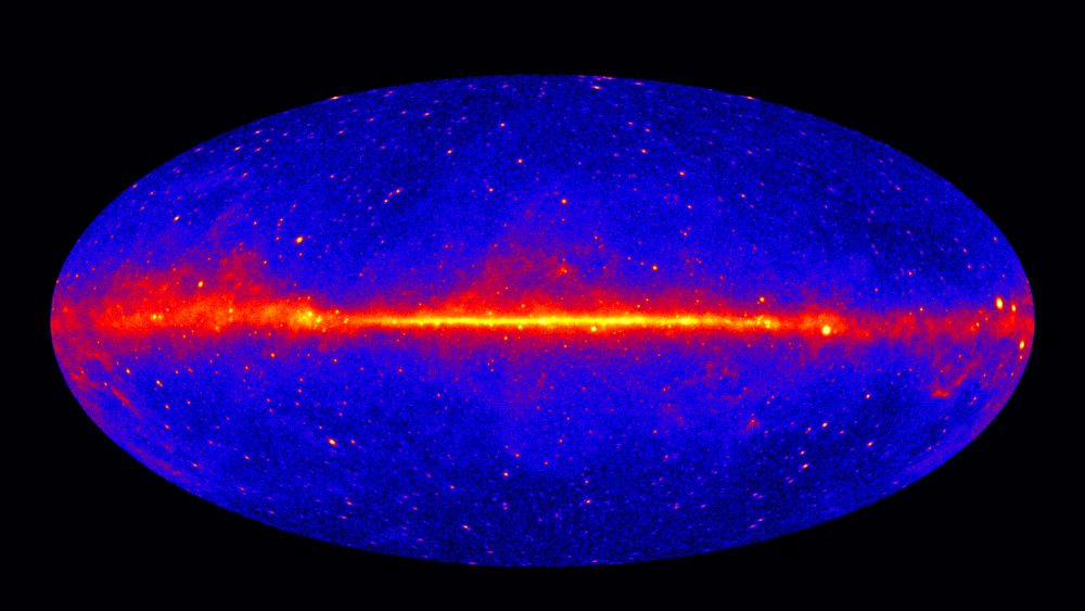
Figure 4:Skymap in Galactic coordinates of the excess of gamma-rays with energies above GeV from 5 years of observations with Fermi-LAT. From this page.
Most of the sources observed at GeV energies are located outside the Galactic Plane. They are mainly jetted active galactic nuclei, the brightest of which are “blazars”, whose axis of emission is aligned with the line of sight. Other jetted active galactic nuclei with a “misaligned” jet are called radio galaxies. Approximately a dozen starburst galaxies have also been detected in the extragalactic universe observed in gamma rays. These galaxies exhibit a higher rate of star formation per unit of stellar mass than our own galaxy. With respect to the Milky Way, starburst galaxies produce more short-lived, massive stars that end their lives in supernovae. Several hundred gamma-ray bursts have also been detected in the extragalactic gamma-ray sky, primarily long gamma-ray bursts resulting from the explosions of massive stars up to a redshift of .
Diffuse emissions from our galaxy can be seen firstly along the Galactic plane and secondly as a fainter peanut-shaped emissions on either side of the Galactic centre: the Fermi bubbles. These bubbles have a similar morphology to those observed in microwaves by the WMAP and Planck satellites and in X-rays by the eROSITA satellite. The mainstream explanation for the Fermi bubbles is the past acceleration of cosmic rays in the inner regions of the Milky Way, followed by the diffusion of these charged particles in the Galactic magnetic field.
Finally, our galaxy is populated by a myriad of stellar-sized sources. Hollow shells are the remains of supernovae (of which there are two types: core-collapse and thermonuclear, also known as SN1a). Core-collapse supernovae can leave a highly magnetised neutron star in their core after their explosion, which is known as a pulsar. The winds from these pulsars, known as pulsar wind nebulae, fill the space left by the supernova explosion and accelerate electrons and positrons, which re-radiate gamma rays. In more advanced stages of their lives, the diffusion of particles around the pulsar can even lead to extended emission over several degrees, known as TeV halos. Our galaxy also contains numerous gamma-ray sources arising from binary systems: novae, X-ray binaries and even microquasars, which are the stellar-scale analogues of the jetted active galactic nuclei.
Static images, such as those presented in Figure 2 and Figure 3, are particularly useful for astronomical sources that are periodic or constant on human timescales. For such sources, observations at different wavelengths made at different times can be combined a posteriori without altering the physical picture. However, this does not apply to persistent variable sources, such as a jetted active galactic nucleus, the flux of which varies erratically on timescales ranging from decades to minutes, nor to transient sources, such as gamma-ray bursts and novae, which appear and disappear within seconds to days after explosions.
Fortunately, since the early 2020s, we have had access to a network of multi-wavelength observatories covering nearly 22 orders of magnitude in energy, from a few tens of MHz to energies on the order of PeV, including some with spectroscopic or polarimetric capabilities. Simultaneous observation campaigns are scheduled and bursts can be followed up thanks to alerts transmitted worldwide within minutes. These alerts are also issued by multi-messenger facilities, which have been crucial since the mid-2010s as we will discuss in the next lesson.
Relativistic beaming
The most variable sources known to date often display (or are inferred to host) jets of plasmas.
The existence of emission zones with a bulk velocity (relative to the central compact object) approaching the speed of light can be illustrated by the apparent motion of plasma region (often called “blobs”) in such astrophysical jets. The apparent velocity of such plasma blobs can exceed the speed of light, an effect that can be explained by purely geometrical arguments based on classical physics, as Exercise 1 illustrates.
Solution to Exercise 1
Following the notations in figure 6, the apparent velocity, , of the plasma blob is given by
where is the physical speed of the plasma blob along the jet in the observer’s frame.
Using and , together with standard trigonometry gives:
So that after a bit of algebra, an apparent speed that is equal to a fraction of the speed of light reads
where is the Lorentz factor of the plasma blob.
The right-hand-side equation has a solution if and only if i.e. . As and , one gets i.e. a Lorentz factor larger than 4 for the jet of the active galactic nucleus 3C 279.
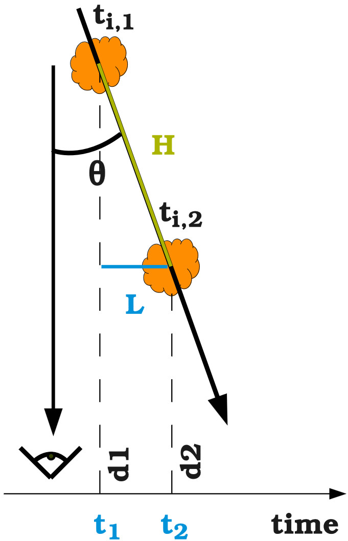
Figure 6:Schematic modeling of the radio knot.
The relativistic motion of the plasma blobs in jetted astrophysical sources results in anisotropic emission. The motion also increases the energy of the photons and the intensity of the radiation as the region moves towards the observer. The textbook derivation of this relativistic Doppler effect is based on velocity transformations. Alternatively, we use here a more straightforward approach based on the transformation of the energy of an emitted photon.
Assume an isotropic emission of energy in the frame that is comoving with the emitting region, with corresponding four-momentum . The observer receives photons of energy in the lab frame along the direction, so the observed four-momentum is . We can go from one frame to the other via a Lorentz-boost of the emitting region and a rotation by an angle from the direction of motion, i.e.
The first space-like component reads . Photons emitted in the forward direction thus reach the observer within a cone defined by . In the ultra-relativistic limit, this inequality reads , which defines a cone of half-opening angle . This corresponds to a half-opening angle .
The time-like component equation reads . Thus, in the observer’s frame, the energy is enhanced by a Doppler factor i.e.
This increase in energy corresponds to an increase in frequency and therefore to a shortening of the observed time scales by a factor . In the ultra-relativistic limit and for a jet nearly aligned with the line of site (blazar-like source), this correspond to an energy enhancement or a time shortening by a factor that is .
The specific intensity of the source, i.e. its brightness, is also enhanced. As is Lorentz invariant, the specific intensity is enhanced by a factor and the bolometric intensity, , is enhanced by a factor .
Solution to Exercise 2
Each shell reaches a radius , with and . The internal shock occurs at a distance and time . Then, , i.e.
The optical depth is the product of a distance, a target density and a cross section. This pure number that quantifies the probability of interaction is Lorentz invariant. We can calculate its value in the isotropic emission frame: , where the distance is (causality argument) and where target photon density is . This yields an optical depth:
The region is partly transparent to photons for , i.e. for
which corresponds to in the ultrarelativistic limit.
Injecting this lower bound on the Lorentz factor into the solution to question 1 yields m i.e. about 1 A.U.
- Rybicki, G. B., & Lightman, A. P. (1986). Radiative Processes in Astrophysics.
- Fukugita, M., & Peebles, P. J. E. (2004). The Cosmic Energy Inventory. \apj, 616(2), 643–668. 10.1086/425155
- Biteau, J. (2025). Cosmic inventory of the background fields of relativistic particles in the Universe. arXiv E-Prints, arXiv:2509.17954. 10.48550/arXiv.2509.17954
- Aharonian, F., Ait Benkhali, F., Aschersleben, J., Ashkar, H., Backes, M., Baktash, A., Barbosa Martins, V., Batzofin, R., Becherini, Y., Berge, D., Bernlöhr, K., Bi, B., Böttcher, M., Boisson, C., Bolmont, J., de Bony de Lavergne, M., Borowska, J., Bradascio, F., Breuhaus, M., … Harding, A. (2024). Spectrum and extension of the inverse-Compton emission of the Crab Nebula from a combined Fermi-LAT and H.E.S.S. analysis. \aap, 686, A308. 10.1051/0004-6361/202348651